
In my study, I treat gear hobbing as the central generating process that connects tool motion, workpiece motion, tooth profile formation, and final transmission behavior. I begin from the observation that gear hobbing is not simply a shaping operation. It is a continuous generating process in which the cutting edges of a hob and the tooth spaces of the workpiece maintain a strict conjugate relationship. When this relationship is disturbed by any error source, the resulting gear no longer matches the ideal involute geometry. The disturbance changes the instantaneous meshing point, the nodal position, the pressure angle, the tooth thickness, and the local contact condition. My aim is to connect these changes in a single analytical and numerical framework, so that gear hobbing errors can be mapped to parametric models and then evaluated through static and transient contact analysis.
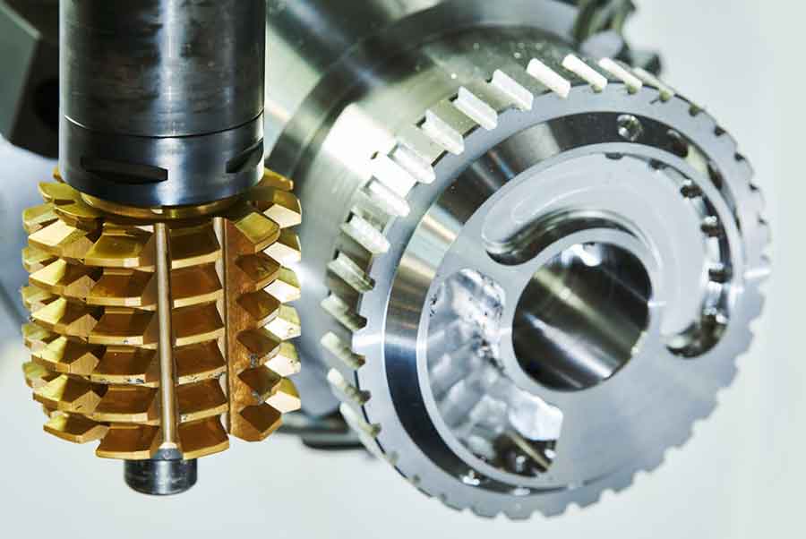
From my perspective, the most useful way to study gear hobbing accuracy is to separate the error sources according to their origin and their frequency. Large periodic errors mainly affect transmission accuracy, while small periodic errors mainly affect smoothness and noise. In gear hobbing, the harmonic order relative to one workpiece revolution is a practical criterion. When the harmonic order is below four, I classify the effect as a large periodic error. When it is above four, I classify it as a small periodic error. The harmonic order does not have to be an integer, because some errors, such as worktable spindle runout, can create a half-order component.
| Error class | Typical source in gear hobbing | Dominant effect |
|---|---|---|
| Large periodic systematic error | Geometric eccentricity, kinematic eccentricity, low-frequency spindle and chain error | Transmission accuracy, cumulative pitch error, radial runout |
| Small periodic systematic error | High-frequency spindle error, transmission chain ripple, tool manufacturing error | Profile error, pitch deviation, smoothness, noise |
| Random error | Cutting force variation, thermal deformation, wear, fixture disturbance | Scattered profile and pitch deviations, unstable contact |
| Tool error | Hob profile angle error, pitch error, helix error, installation error | Tooth profile distortion, asymmetric flanks, thickness bias |
| Motion error | Worktable rotation error, hob spindle rotation error, transmission chain error | Instantaneous mesh point shift, kinematic eccentricity |
I describe the generating relation of gear hobbing by replacing the hob with an equivalent rack for the straight cutting edge. This simplification is valid because the active cutting edge of a hob can be treated as a rack tooth profile in the normal section. The rack and the gear maintain a pure rolling relation between the rack pitch line and the gear pitch circle. If the rack moves a distance equal to the arc length on the pitch circle, the gear rotation angle is determined. I write the nodal radius vector in the gear coordinate system as
$$ \mathbf{r} = r(\cos\phi\,\mathbf{i}_2 + \sin\phi\,\mathbf{j}_2). $$
The rack displacement is then
$$ P_1O = vt = r\phi. $$
The corresponding normal distance and vector relation are
$$ O_1N = P_1O\sin\alpha = r\phi\sin\alpha, $$
$$ \mathbf{O_1N} = -r\phi\sin\alpha\,\mathbf{i} + r\phi\cos\alpha\,\mathbf{j}. $$
After the gear rotates by an angle, the generating point in the fixed coordinate system is obtained by vector addition. The ideal tooth profile in the gear-fixed coordinate system reduces to the standard involute form
$$ \mathbf{r}_c = r_b[\cos\theta + (\theta-\alpha)\sin\theta]\mathbf{i}_2 + r_b[\sin\theta – (\theta-\alpha)\cos\theta]\mathbf{j}_2, $$
where
$$ r_b = r\cos\alpha. $$
This result is important for gear hobbing because it shows that the ideal generated profile is determined by the base radius and the pressure angle. Any gear hobbing error that changes the effective pressure angle or the effective center distance will change the base radius and therefore the entire involute.
I then examine eccentricity error. In gear hobbing, eccentricity appears in two main forms: geometric eccentricity and kinematic eccentricity. Geometric eccentricity arises when the workpiece center hole, fixture mandrel, and worktable rotation axis do not coincide. Kinematic eccentricity arises when the indexing worm wheel or another transmission element introduces a periodic angular velocity variation. Both errors change the instantaneous nodal position. For geometric eccentricity, the instantaneous node moves from the ideal point to a new point on the line of action. The induced profile increment is
$$ \Delta r_c = NN’ = PP’ = e_g. $$
The gear-fixed vector of geometric eccentricity is
$$ \mathbf{e}_g = e_g(\cos\phi\,\mathbf{i} + \sin\phi\,\mathbf{j}). $$
In the gear coordinate system this becomes
$$ \mathbf{e}_g = e_g\mathbf{i}_2. $$
Therefore, the actual profile equation can be written as
$$ \mathbf{r}_c’ = \mathbf{r}_c + \mathbf{e}_g. $$
I find that geometric eccentricity maps almost one-to-one into the generated gear. The profile remains involute in a local sense, but the base circle is shifted. The center of the base circle no longer coincides with the rotation center.
For kinematic eccentricity, I consider an indexing worm wheel with eccentricity \(e_w\). If the ideal rotation angle is \(\phi_0\), the actual rotation angle is
$$ \phi = \phi_0 – e\sin\phi, $$
where
$$ e = \frac{e_w}{r_w}. $$
Differentiating with respect to time gives the angular velocity ratio
$$ \omega = \frac{\omega_0}{1+e\cos\phi}. $$
The instantaneous nodal radius becomes
$$ r’ = r(1+e\cos\phi). $$
The kinematic eccentricity projected onto the base circle is
$$ e_m = r_b e = r e \cos\alpha. $$
Thus, kinematic eccentricity also leaves the local profile as an involute, but it shifts the base circle. The difference is that its mapping ratio is not one-to-one. It depends on the ratio of the worm wheel radius to the gear pitch radius and on the pressure angle.
When geometric and kinematic eccentricities coexist, I combine them as vectors. The left-flank and right-flank eccentricities are
$$ e_L = \sqrt{e_g^2+e_m^2+2e_g e_m\cos(\psi-\alpha)}, $$
$$ e_R = \sqrt{e_g^2+e_m^2+2e_g e_m\cos(\psi+\alpha)}. $$
The corresponding phase angles are
$$ \tan\gamma_L = \frac{e_m\sin(\psi-\alpha)}{e_g+e_m\cos(\psi-\alpha)}, $$
$$ \tan\gamma_R = \frac{e_m\sin(\psi+\alpha)}{e_g+e_m\cos(\psi+\alpha)}. $$
This synthesis is helpful because it explains why the two flanks of a gear produced by gear hobbing can respond differently to the same underlying eccentricity. If only geometric eccentricity exists, the two flanks have equal magnitude. If only kinematic eccentricity exists, the two flanks have equal magnitude but opposite phase shifts. When both exist, the left and right flanks can become unequal.
| Error source | Physical cause in gear hobbing | Profile consequence | Mapping behavior |
|---|---|---|---|
| Geometric eccentricity | Workpiece, fixture, and worktable axes do not coincide | Base circle shift, radial runout | Nearly one-to-one |
| Kinematic eccentricity | Indexing worm wheel or transmission element eccentricity | Base circle shift, periodic angular error | Scaled by radius ratio and pressure angle |
| Worktable spindle runout | Main spindle rotation error | Similar to geometric eccentricity | Low-frequency component dominates |
| Hob spindle runout | Tool spindle radial and axial error | Profile, pitch, and lead deviations | Contains multiple harmonics |
| Transmission chain error | Gear, worm, screw, and bearing errors | Periodic rotation error | Superposition of many components |
I also analyze spindle rotation error. For the worktable spindle, the actual rotation center is displaced from the theoretical center. The instantaneous node changes in a way similar to geometric eccentricity. The profile increment is again
$$ \Delta r_c = NN’ = PP’ = e_r. $$
For the hob spindle, the error has both radial and axial components. I express the radial and tangential components as Fourier series:
$$ e_y = e_{y0} + \sum_j e_{yj}\sin(j\phi+\psi_{yj}), $$
$$ e_z = e_{z0} + \sum_j e_{zj}\sin(j\phi+\psi_{zj}). $$
The low-frequency components of spindle error produce large periodic errors, while the high-frequency components produce small periodic errors. In gear hobbing, this distinction is critical because the same spindle error spectrum can affect both transmission accuracy and tooth surface smoothness.
Transmission chain error is another major contributor. In gear hobbing, the internal transmission chain connects the hob rotation and the workpiece rotation. If the \(i\)-th transmission gear has eccentricity \(e_i\), the angular error transmitted to the final workpiece is
$$ \Delta\phi_n = \sum_{i=1}^{n} \frac{e_i}{r_i} m_i \sin(\phi_i+\psi_i), $$
where \(m_i\) is the reciprocal transmission ratio from the \(i\)-th gear to the final gear. The instantaneous nodal radius becomes
$$ r’ = r\left[1+\sum_{i=1}^{n}\frac{e_i}{r_i}m_i\cos(\phi_i+\psi_i)\right]. $$
The resulting profile error behaves like a superposition of many kinematic eccentricity components. This is why transmission chain error is often more complex than a single eccentricity error. It contains multiple frequencies and phases, and its effect on gear hobbing accuracy cannot be reduced to a single scalar value.
Tool error is also central to gear hobbing. The hob profile angle error changes the effective pressure angle. If the profile angle changes by \(d\alpha\), the generated gear remains locally involute, but its base radius changes from \(r\cos\alpha\) to
$$ r_b’ = r\cos(\alpha-d\alpha). $$
The pressure angle at the pitch circle changes from \(\alpha\) to \(\alpha-d\alpha\). This means that a small tool angle error can shift the contact position along the line of action. The resulting profile error is not a simple offset. It is a rotation of the involute about the base circle.
For hob installation error, I focus on three factors: radial runout \(\Delta r\), axial shift \(\Delta b\), and mounting axis angle error \(\Delta\delta\). Radial runout effectively changes the center distance. The generated gear behaves like a slightly shifted or modified gear, with an equivalent modification coefficient
$$ x_m = \frac{\Delta r}{m}. $$
Axial shift is more complicated because it depends on the hob rotation angle. It can be one-directional or two-directional. In two-directional shift, the hob moves back and forth and returns to its original position after one revolution. The resulting error is periodic and can be expressed as a function of hob rotation. Mounting axis angle error tilts the hob axis relative to its ideal position. It changes the two flanks in opposite directions:
$$ \alpha_L = \alpha+\Delta\delta, \qquad \alpha_R = \alpha-\Delta\delta. $$
Therefore, the two flanks of the generated gear have different effective pressure angles, and the tooth becomes asymmetric. This asymmetry affects both contact stress and bending stress.
| Hob installation error | Symbol | Primary geometric effect | Gear hobbing consequence |
|---|---|---|---|
| Radial runout | \(\Delta r\) | Center distance variation | Tooth thickness change, equivalent modification |
| Axial shift | \(\Delta b\) | Axial position variation | Pitch and profile ripple |
| Mounting axis angle error | \(\Delta\delta\) | Axis tilt | Asymmetric flanks, pressure angle difference |
To build a parametric model, I derive the tooth profile from the gear hobbing coordinate transformation. I define the hob coordinate system \(Px_0y_0\) and the gear coordinate system \(Oxy\). The hob coordinate system is attached to the cutting edge, while the gear coordinate system rotates with the workpiece. The general transformation from the hob coordinate to the gear coordinate is
$$ \begin{bmatrix} x \\ y \end{bmatrix} = \begin{bmatrix} \cos\phi & -\sin\phi \\ \sin\phi & \cos\phi \end{bmatrix} \begin{bmatrix} x_0-r \\ y_0 \end{bmatrix} + \begin{bmatrix} r\cos\phi \\ r\sin\phi \end{bmatrix}. $$
Here \(\phi\) is the rolling angle of the generating motion. For the involute part, the cutting edge is a straight line. For the transition part, the cutting edge is a circular arc. For the root part, the cutting edge is the top edge. I divide the hob profile into these three segments and derive the corresponding profile equations.
The involute part is generated by the straight edge. If the straight edge point is \((x_0,y_0)\), the point in the gear coordinate system is obtained from the transformation above. The standard involute equation can then be written as
$$ x = r_b(\cos t + t\sin t), \qquad y = r_b(\sin t – t\cos t). $$
The transition curve is generated by the circular arc of the hob tip. If the arc center is \((x_c,y_c)\) and the arc radius is \(r_0\), a point on the arc is
$$ x_0 = x_c + r_0\cos\gamma, \qquad y_0 = y_c – r_0\sin\gamma. $$
The angle \(\gamma\) is measured from the normal to the cutting edge. The root curve is generated by the top edge. Its coordinates can be written as
$$ x_0 = x_{b0} – (r-r_{b0})\sin(\phi-\delta), $$
$$ y_0 = y_{b0} + (r-r_{b0})\cos(\phi-\delta). $$
For a helical gear, the end profile is rotated along the tooth width. If the rotation angle at a given section is \(\theta\), then
$$ \theta = \frac{z}{r}\tan\beta, $$
and the helical surface is obtained by rotating the end profile:
$$ \begin{bmatrix} x’ \\ y’ \\ z’ \end{bmatrix} = \begin{bmatrix} \cos\theta & -\sin\theta & 0 \\ \sin\theta & \cos\theta & 0 \\ 0 & 0 & 1 \end{bmatrix} \begin{bmatrix} x \\ y \\ z \end{bmatrix}. $$
Using these equations, I create a parametric model in a CAD environment. I use a table of driving parameters to control the model. The basic gear parameters are listed below.
| Parameter | Symbol | Value |
|---|---|---|
| Normal module | \(m_n\) | 3 mm |
| Number of teeth | \(z\) | 20 |
| Pressure angle | \(\alpha\) | 20° |
| Helix angle | \(\beta\) | 8° |
| Face width | \(b\) | 12 mm |
| Addendum coefficient | \(h_a^*\) | 1 |
| Clearance coefficient | \(c^*\) | 0.25 |
I implement the parametric gear hobbing model through expressions, curves, sweep features, and a custom dialog. The expressions control the involute, transition curve, root curve, and helix. I create a menu and a dialog so that the user can input the module, tooth number, helix angle, face width, radial runout, and mounting axis angle error. The model updates automatically after the input values change. This is a practical way to connect gear hobbing error theory with a parametric solid model.
To evaluate the effect of hob installation error, I compare four profile models: no error, mounting axis angle error only, radial runout only, and both errors together. The tooth thickness at the base circle, pitch circle, and addendum circle changes with the error state. I calculate the tooth thickness using the involute function
$$ \text{inv}\,\alpha = \tan\alpha – \alpha. $$
The thickness at an arbitrary circle is
$$ s_x = d_x\left(\frac{\pi}{z}+\text{inv}\,\alpha-\text{inv}\,\alpha_x\right). $$
The base circle thickness is
$$ s_b = d_b\left(\frac{\pi}{z}+\text{inv}\,\alpha\right). $$
The pitch circle thickness for a standard gear is
$$ s = \frac{\pi m}{2}. $$
The addendum circle thickness is
$$ s_a = d_a\left(\frac{\pi}{z}+\text{inv}\,\alpha-\text{inv}\,\alpha_a\right). $$
The comparison of tooth thickness is summarized below.
| Model | Base circle thickness (mm) | Pitch circle thickness (mm) | Addendum circle thickness (mm) |
|---|---|---|---|
| No error | 5.37815 | 4.78509 | 2.14078 |
| Angle error only | 5.37864 | 4.78880 | 2.13824 |
| Radial runout only | 5.17068 | 4.56332 | 1.89710 |
| Both errors | 5.16632 | 4.56673 | 1.89430 |
I observe that radial runout reduces tooth thickness significantly, especially near the addendum. This weakens the tooth and changes the contact path. Mounting axis angle error makes the two flanks asymmetric. When both errors exist, the tooth becomes thinner and asymmetric. In gear hobbing, this means that the generated gear may appear acceptable in overall size but fail in local contact and bending performance.
After parametric modeling, I perform static contact analysis. The contact problem between gear teeth is nonlinear because the contact area, contact pressure, and sliding state change during meshing. I use a penalty-based augmented Lagrangian method to enforce contact compatibility. The classical Hertz theory provides a reference for the maximum contact stress between two cylinders. For two elastic cylinders in line contact, the maximum contact stress is
$$ \sigma_H = \sqrt{\frac{F_n}{\pi L \rho} \frac{1}{\frac{1-\mu_1^2}{E_1}+\frac{1-\mu_2^2}{E_2}}}. $$
For a gear pair, the equivalent curvature radius at the instantaneous contact point is
$$ \rho = \frac{\rho_1\rho_2}{\rho_1+\rho_2}. $$
The contact stress formula used in gear design can be written as
$$ \sigma_H = Z_E Z_H Z_\epsilon Z_\beta \sqrt{\frac{K T_1 (u+1)}{b d_1^2 u}}. $$
I also calculate the overlap ratios. The transverse contact ratio is
$$ \epsilon_\alpha = \left[1.88-3.2\left(\frac{1}{z_1}+\frac{1}{z_2}\right)\right]\cos\beta. $$
The overlap ratio is
$$ \epsilon_\beta = \frac{b\sin\beta}{\pi m_n}. $$
The total contact ratio is
$$ \epsilon_\gamma = \epsilon_\alpha+\epsilon_\beta. $$
For the gear pair in my model, the total contact ratio is about 1.72. This means that the gear pair operates in alternating single-tooth and double-tooth contact. The maximum contact stress occurs near the pitch point during single-tooth contact.
For the static contact analysis, I import four gear meshing models into the finite element environment. Each model contains an active gear and a driven gear. The active gear has a hinge constraint with rotational freedom, and the driven gear has a fixed hinge constraint. A torque of 50 N·m is applied to the active gear. A frictional contact pair is created between the mating flanks. The friction coefficient is 0.2. The mesh is generated with hex-dominant elements, and the contact region is refined. The material is structural steel. The interface treatment is set to adjust to touch, so that initial gaps or penetrations do not create artificial stresses.
| Gear pair | Active gear error | Driven gear error |
|---|---|---|
| A | \(\Delta r=0,\ \Delta\delta=0^\circ\) | \(\Delta r=0,\ \Delta\delta=0^\circ\) |
| B | \(\Delta r=0,\ \Delta\delta=0.2^\circ\) | \(\Delta r=0,\ \Delta\delta=0.2^\circ\) |
| C | \(\Delta r=0.1\,\text{mm},\ \Delta\delta=0^\circ\) | \(\Delta r=0.1\,\text{mm},\ \Delta\delta=0^\circ\) |
| D | \(\Delta r=0.1\,\text{mm},\ \Delta\delta=0.2^\circ\) | \(\Delta r=0.1\,\text{mm},\ \Delta\delta=0.2^\circ\) |
The static contact results are summarized below. The equivalent stress and contact stress are compared for the four models.
| Gear pair | Equivalent stress (MPa) | Contact stress (MPa) |
|---|---|---|
| A | 466.57 | 569.03 |
| B | 495.47 | 567.66 |
| C | 454.81 | 563.01 |
| D | 475.83 | 572.09 |
I find that the equivalent stress is more sensitive to hob installation error than the maximum contact stress in static analysis. Compared with the ideal gear pair, the angle-error model increases the maximum equivalent stress by about 6.2%, the radial-runout model decreases it by about 2.5%, and the combined-error model increases it by about 2.0%. The maximum contact stress changes by less than 1.1% in all cases. This does not mean that the contact condition is safe. The local contact state can deteriorate even when the peak contact stress changes only slightly. The contact area may shift toward the tooth tip or root, and the load distribution may become uneven along the face width.
I also examine the tooth root condition. Radial runout can produce undercut or a thinner root. Mounting axis angle error can make the root curve asymmetric. Both effects reduce the bending fatigue strength. In gear hobbing, these errors are not independent. They are generated by the same installation process and often appear together. Therefore, a model that includes only one error source may underestimate the risk.
Next, I perform transient dynamic contact analysis. The static analysis cannot capture inertia, damping, impact, or the time-dependent contact state. The governing equation for structural dynamics is
$$ [M]\{\ddot{x}\}+[C]\{\dot{x}\}+[K]\{x\}=\{F(t)\}. $$
Here \([M]\), \([C]\), and \([K]\) are the mass, damping, and stiffness matrices. The vectors \(\{\ddot{x}\}\), \(\{\dot{x}\}\), and \(\{x\}\) are acceleration, velocity, and displacement. \(\{F(t)\}\) is the time-dependent load vector. I use the full method for the transient analysis because it can handle nonlinear contact and large motion. The Rayleigh damping model is
$$ [C]=\alpha[M]+\beta[K]. $$
The damping ratio is related to the Rayleigh coefficients by
$$ \zeta = \frac{\alpha}{2\omega}+\frac{\beta\omega}{2}. $$
For the transient analysis, I apply an angular displacement of 22° to the active gear. The default time is 1 s, so the angular velocity is about 0.384 rad/s. A torque of 50 N·m is applied to the driven gear. The initial time step is chosen from the modal result:
$$ \Delta t_{ini} = \frac{1}{20f_{res}}. $$
I set the initial number of substeps to 30, the minimum to 10, and the maximum to 100. Automatic time stepping is used to balance accuracy and computational cost. The transient results show clear single-tooth and double-tooth contact regions, with impact peaks during the transition between them.
| Gear pair | Static contact stress (MPa) | Transient maximum contact stress (MPa) | Single-tooth average contact stress (MPa) | Double-tooth average contact stress (MPa) | Maximum impact stress (MPa) |
|---|---|---|---|---|---|
| A | 569.03 | 621.06 | 608.11 | 384.05 | 925.81 |
| B | 567.66 | 592.78 | 571.62 | 337.23 | 859.03 |
| C | 563.01 | 585.71 | 565.01 | 351.01 | 917.16 |
| D | 572.09 | 629.57 | 608.65 | 385.06 | 939.80 |
I find that the transient maximum contact stress is about 6.9% higher on average than the static maximum contact stress. This is expected because the transient analysis includes inertia and damping, and because the contact point moves across the tooth flank during meshing. The impact stress is much higher than the average contact stress, especially during the transition from double-tooth contact to single-tooth contact. This impact behavior is important in gear hobbing because small profile deviations can shift the impact location and increase the dynamic load.
When only one error factor exists, the contact stress and impact stress may decrease. For example, gear pair B has a smaller transient maximum contact stress and a smaller impact stress than gear pair A. Gear pair C also has a smaller transient maximum contact stress than gear pair A. However, I do not interpret this as an improvement. The reason is that the single error factor acts like an unintended modification. It changes the tooth profile in a way that may reduce the local peak stress at one point, but it also destroys the normal meshing state and damages the root region. The modification is not designed for load sharing. It does not produce a smooth contact path. It can make the contact concentrated near the tip or root and reduce the bending fatigue strength.
When both error factors exist, the contact stress and impact stress increase. Gear pair D has the highest static contact stress, the highest transient maximum contact stress, and the highest maximum impact stress among the four models. Since real gear hobbing almost always includes both radial runout and mounting axis angle error, the combined case is the most representative. This is the main practical conclusion I draw from the dynamic analysis.
I summarize the main mapping rules from error source to gear performance below.
| Error source in gear hobbing | Profile effect | Contact effect | Dynamic effect |
|---|---|---|---|
| Geometric eccentricity | Base circle shift | Uneven load around the gear | Low-frequency transmission error |
| Kinematic eccentricity | Periodic base circle shift | Cyclic contact variation | Angular velocity ripple |
| Worktable spindle runout | Radial profile deviation | Contact position shift | Low-frequency vibration |
| Hob spindle runout | Multiple harmonic profile error | Local contact concentration | High-frequency excitation |
| Transmission chain error | Superposed periodic profile error | Time-varying contact load | Complex frequency response |
| Tool profile angle error | Base radius change | Pressure angle shift | Change in contact timing |
| Hob radial runout | Tooth thickness change | Contact area change | Impact stress change |
| Hob axis angle error | Asymmetric flanks | One-sided contact | Increased impact |
From my point of view, the most important practical step in gear hobbing quality control is to reduce the combined installation error of the hob. Radial runout changes the effective center distance and tooth thickness. Mounting axis angle error changes the pressure angle on each flank and makes the gear asymmetric. When these errors are present, the generated gear may still pass a simple dimensional check, but its contact and bending behavior can be poor. The finite element results show that the combined error increases the static contact stress, transient maximum contact stress, average single-tooth contact stress, average double-tooth contact stress, and maximum impact stress. This is a clear warning for high-speed and heavy-load gear systems.
I also note that gear hobbing is closely related to gear grinding in terms of generating kinematics. The same coordinate transformation and error mapping ideas can be extended from gear hobbing to profile grinding. In both processes, the final tooth surface is the envelope of the tool cutting edge under a prescribed generating motion. Therefore, the error analysis developed here is not limited to gear hobbing alone. It provides a general method for connecting tool installation errors, generating motion errors, tooth profile deviations, and loaded contact behavior.
For parametric modeling, I recommend using the following workflow in gear hobbing research. First, define the ideal generating kinematics and derive the ideal tooth profile. Second, introduce the dominant error parameters, such as radial runout and axis angle error. Third, express the tooth profile as a function of these parameters. Fourth, build the solid model through a parametric CAD platform. Fifth, export the model to a finite element environment. Sixth, perform static and transient contact analysis under realistic boundary conditions. Seventh, compare the stress, contact area, impact, and deformation results with the ideal case. This workflow allows the effect of gear hobbing errors to be evaluated before physical manufacturing.
The equations and tables in my study support several conclusions. The ideal gear hobbing process generates an involute profile determined by the base radius. Eccentricity errors preserve the local involute shape but shift the base circle. Spindle errors and transmission chain errors create periodic nodal shifts. Tool profile angle errors change the effective pressure angle and base radius. Hob installation errors change tooth thickness and flank symmetry. These geometric changes alter the contact stress and bending stress. Static contact analysis shows that the equivalent stress is more sensitive than the maximum contact stress to single error factors, while the combined error increases both stresses. Transient contact analysis shows that inertia, damping, and impact raise the maximum contact stress by about 6.9% on average. The combined installation error produces the highest dynamic stress and impact stress.
In my future work, I would extend the model in three directions. First, I would include multiple error sources simultaneously, rather than treating each source separately. The interaction between geometric eccentricity, kinematic eccentricity, spindle runout, transmission chain error, and hob installation error is nonlinear and may produce unexpected contact states. Second, I would include elastic deformation, thermal deformation, and dynamic transmission error in the finite element model. These effects are important in high-speed gear hobbing and in precision gear transmission. Third, I would include assembly error in the gear pair model. A gear that is accurate after gear hobbing can still perform poorly if the assembly axis is misaligned. A complete accuracy chain should connect gear hobbing, measurement, assembly, and operation.
Overall, I see gear hobbing error modeling as a bridge between manufacturing and performance. The manufacturing error is not just a dimensional deviation. It changes the generating geometry, the tooth surface, the contact path, the load distribution, and the dynamic response. By combining analytical mapping, parametric modeling, and finite element analysis, I can quantify how gear hobbing errors affect gear behavior. This approach helps explain why two gears with similar overall dimensions can have very different noise, vibration, contact fatigue life, and bending fatigue life. It also provides a basis for error compensation, process improvement, and high-precision gear design.