
I have focused my research on the design, modification, and nonlinear dynamic behavior of a helical gear pair used in an automotive transmission. My aim has been to improve transmission smoothness, reduce vibration and noise, and provide a practical framework for selecting tooth profile modification parameters. A helical gear system is widely used because it offers high transmission efficiency, compact structure, and gradual meshing. However, manufacturing errors, assembly deviations, elastic deformation under load, and sudden changes in meshing force can still produce impact, uneven load distribution, and undesirable dynamic response. In my work, I combine parametric modeling, finite element modal analysis, response surface methodology, transmission error verification, software development, and nonlinear dynamic analysis to study the helical gear system in a systematic way.
The helical gear pair I studied has a normal module of 4 mm, a helix angle of 16.835 degrees, and a pressure angle of 19 degrees. The driving gear has 23 teeth, and the driven gear has 44 teeth. The face widths are 24 mm and 22 mm, respectively. These values are summarized in the table below. I used these parameters as the baseline for all later finite element simulations, modification experiments, and dynamic calculations.
| Parameter | Driving helical gear | Driven helical gear |
|---|---|---|
| Number of teeth | 23 | 44 |
| Helix angle (degree) | 16.835 | 16.835 |
| Pressure angle (degree) | 19 | 19 |
| Normal module (mm) | 4 | 4 |
| Face width (mm) | 24 | 22 |
| Pitch diameter (mm) | 96.1 | 183.9 |
For the geometric modeling of the helical gear, I first defined the involute profile in the transverse plane. The involute is generated by a straight line rolling without slipping on a base circle. For a point on the involute, the Cartesian coordinates can be written as follows:
$$x = r_b(\cos u + u\sin u)$$
$$y = r_b(\sin u – u\cos u)$$
Here, the base circle radius is determined by the normal module, the number of teeth, and the pressure angle:
$$r_b = \frac{m z}{2}\cos\alpha$$
The parameter u is related to the pressure angle and the involute angle. The maximum value of u occurs when the involute reaches the addendum circle. I used a parametric equation approach in a three-dimensional CAD environment so that the helical gear model could be regenerated quickly when the tooth number, module, helix angle, or pressure angle changed. This parametric strategy was important because I needed to create several modified helical gear models for the response surface experiments. A helical gear is not simply a spur gear extruded along its axis; the tooth profile is swept along a helical line. Therefore, I generated the transverse involute, created the helical sweep path, and then cut the tooth space. The tooth space was patterned around the gear axis to form the complete helical gear.
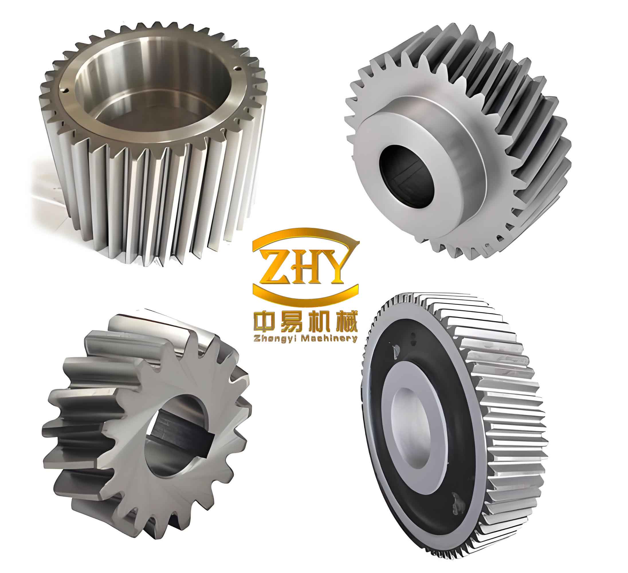
After building the driving and driven helical gears, I assembled them with the correct center distance and helix direction. The assembled helical gear pair was saved in a neutral format and imported into finite element software. The material assigned to the helical gear was 20CrMnTi, a common carburizing steel for transmission gears. I defined the elastic modulus, Poisson ratio, and density in the engineering data module. The contact between the driving and driven tooth surfaces was set as frictional contact with a friction coefficient of 0.2. I refined the mesh on the contact and target surfaces while allowing a coarser mesh in regions far from the contact zone. This approach reduced computation time without sacrificing accuracy in the contact region.
Modal analysis was performed to study the natural characteristics of the helical gear system. For a linear multi-degree-of-freedom system, the governing equation without external force and damping can be expressed as:
$$[M]\{\ddot{q}(t)\} + [K]\{q(t)\} = 0$$
where M is the mass matrix, K is the stiffness matrix, and q is the generalized displacement vector. The solution leads to natural frequencies and mode shapes. I used the Block Lanczos method because it is robust and efficient for large finite element models. The first fifteen natural frequencies were extracted. The lowest natural frequency was approximately 3297.9 Hz, and the fifteenth natural frequency was approximately 12544 Hz. The maximum meshing frequency under the operating speed was lower than the lowest natural frequency, so I concluded that the helical gear system would not resonate under normal working conditions.
The mode shapes showed that the driven helical gear exhibited more significant torsional deformation in the lower modes. Several modes were dominated by rotation of the driven gear about its axis, while the later modes involved more motion of the driving gear. This information was useful because it indicated which part of the helical gear pair might be more sensitive to dynamic excitation. The modal results also provided a reference for later dynamic modeling. A summary of the first fifteen natural frequencies is given in the table below.
| Mode order | Natural frequency (Hz) | Dominant motion description |
|---|---|---|
| 1 | 3297.9 | Torsional motion of driven helical gear |
| 2 | 3765.2 | Driven gear torsional motion with slight axial component |
| 3 | 4218.6 | Driven gear local deformation |
| 4 | 4890.4 | Driven gear torsional motion |
| 5 | 5321.7 | Driven gear bending and torsion |
| 6 | 6058.3 | Driven gear rotation about transverse axis |
| 7 | 6784.1 | Driven gear local mode |
| 8 | 7420.5 | Driven gear torsional mode |
| 9 | 8015.8 | Driven gear torsional mode |
| 10 | 8652.4 | Driven gear deformation |
| 11 | 9240.6 | Driven gear local mode |
| 12 | 9878.2 | Driven gear mode with minor driving gear motion |
| 13 | 10620.7 | Driving gear vibration becomes significant |
| 14 | 11540.3 | Driving gear mode |
| 15 | 12544.0 | Driving gear mode |
After completing modal analysis, I moved to tooth profile modification. In an ideal involute helical gear pair, the load distribution along the contact line should be smooth. In reality, however, the contact ratio is greater than one, and the number of contacting tooth pairs changes during meshing. Single-tooth contact and double-tooth contact alternate. The load carried by each tooth pair changes abruptly at the transition points. This abrupt change causes elastic deformation of the tooth, changes the effective normal pitch, and produces meshing impact. The situation is more complex for a helical gear because contact progresses gradually along the tooth trace, and the total contact ratio includes both transverse and axial components. Nevertheless, proper tooth profile modification can compensate for the deformation and reduce the impact at the beginning and end of meshing.
There are two main categories of gear modification: lead modification and profile modification. Lead modification changes the tooth surface along the face width direction and is mainly used to improve load distribution along the contact line. Profile modification changes the tooth profile in the transverse plane and is mainly used to reduce meshing impact and vibration. I focused on tooth profile modification of the helical gear. The main parameters are the modification curve, the maximum modification amount, and the modification length. I compared several modification curves, including linear, parabolic, exponential, and circular arc forms. The parabolic curve was selected because it can approximate the load deformation curve and avoid sharp discontinuities.
| Modification type | Direction | Typical purpose | Common forms |
|---|---|---|---|
| Lead modification | Along face width | Improve load distribution, reduce edge contact | End relief, helix angle correction, crowning, curved surface |
| Profile modification | Along tooth height | Reduce meshing impact, vibration, and noise | Tip relief, root relief, undercut, parabolic or exponential curve |
For a point on the original involute profile, the coordinates can be transformed to include the modification amount. If the original point is denoted by x and y, the modified point can be written as:
$$x’ = x – \Delta \sin(\alpha_k + \theta_k)$$
$$y’ = y + \Delta \cos(\alpha_k + \theta_k)$$
where the modification amount is denoted by Delta, the pressure angle at the point is denoted by alpha_k, and the involute angle is denoted by theta_k. For a parabolic modification curve, the amount at a given position can be expressed as:
$$\Delta(u) = \Delta_{\max}\left[1 – 1.5\left(\frac{u}{L}\right)^2 + 0.5\left(\frac{u}{L}\right)^3\right]$$
Here, Delta_max is the maximum modification amount, L is the modification length, and u is the position along the modification zone. For an exponential modification curve, I used the following form:
$$\Delta(u) = \Delta_{\max}\left(\frac{u}{L}\right)^n$$
For an arc modification curve, the modification amount can be computed from the radius of the arc and the position along the profile. I also considered empirical methods for estimating the maximum modification amount. One common estimate considers elastic deformation, thermal deformation, and manufacturing error:
$$\Delta_{\max} = \delta + \delta_{\theta} + \delta_m$$
where delta is the elastic deformation under load, delta_theta is the thermal deformation, and delta_m is the manufacturing error. Another practical formula is based on the tangential force, face width, and mesh stiffness:
$$\Delta_{\max} = \frac{K_A F_t}{b C_{\gamma} \varepsilon_{\alpha}}$$
In my study, I used a control variable approach to screen the ranges of the three main modification parameters. I fixed the parabolic coefficient, modification length, or maximum modification amount in turn and evaluated the equivalent stress through finite element contact analysis. The initial screening showed that the maximum modification amount should be studied in the range from 20 to 70 micrometers, the modification length in the range from 3 to 7 mm, and the parabolic curve coefficient in the range from 0.2 to 0.8. These ranges were then used in the response surface design. The control variable results are summarized below.
| Parameter | Fixed value during screening | Screened range |
|---|---|---|
| Maximum modification amount | Curve coefficient 0.4, length 4.8 mm | 20 to 70 micrometers |
| Modification length | Curve coefficient 0.4, amount 40 micrometers | 3 to 7 mm |
| Curve coefficient | Length 4.8 mm, amount 40 micrometers | 0.2 to 0.8 |
I used response surface methodology to optimize the tooth profile modification of the helical gear. Response surface methodology is a statistical and mathematical technique that fits a polynomial relationship between input variables and response values. It is especially useful when multiple parameters interact with each other. I selected a Box-Behnken design because it requires fewer experiments than a full factorial design and can still estimate quadratic effects and interactions. The three factors were the maximum modification amount, the modification length, and the curve coefficient. The responses were the equivalent elastic strain and the equivalent stress obtained from finite element analysis.
| Factor | Symbol | Low level | Middle level | High level |
|---|---|---|---|---|
| Maximum modification amount | A | 20 micrometers | 45 micrometers | 70 micrometers |
| Modification length | B | 3 mm | 5 mm | 7 mm |
| Curve coefficient | C | 0.2 | 0.5 | 0.8 |
The Box-Behnken design generated seventeen simulation cases. For each case, I rebuilt the helical gear pair with the corresponding modification parameters, performed finite element contact analysis, and recorded the maximum equivalent elastic strain and maximum equivalent stress. Before modification, the maximum equivalent stress of the helical gear pair was about 946.46 MPa. After modification, the stress decreased significantly for well-chosen parameters. The design matrix and results are given in the following table.
| Run | A | B | C | Equivalent elastic strain | Equivalent stress (MPa) |
|---|---|---|---|---|---|
| 1 | 20 | 5 | 0.8 | 0.0033674 | 647.25 |
| 2 | 45 | 3 | 0.2 | 0.0032746 | 616.43 |
| 3 | 45 | 5 | 0.5 | 0.0030715 | 537.52 |
| 4 | 45 | 5 | 0.5 | 0.0030784 | 551.77 |
| 5 | 70 | 7 | 0.5 | 0.0034018 | 697.83 |
| 6 | 70 | 3 | 0.5 | 0.0034415 | 726.37 |
| 7 | 70 | 5 | 0.2 | 0.0033305 | 626.48 |
| 8 | 45 | 3 | 0.8 | 0.0033227 | 629.21 |
| 9 | 70 | 5 | 0.8 | 0.0034002 | 658.39 |
| 10 | 45 | 5 | 0.5 | 0.0030732 | 541.22 |
| 11 | 45 | 7 | 0.2 | 0.0032407 | 585.18 |
| 12 | 20 | 7 | 0.5 | 0.0033926 | 682.46 |
| 13 | 20 | 3 | 0.5 | 0.0034379 | 702.94 |
| 14 | 45 | 5 | 0.5 | 0.0030793 | 556.35 |
| 15 | 45 | 7 | 0.8 | 0.0032415 | 602.47 |
| 16 | 45 | 5 | 0.5 | 0.0030778 | 548.28 |
| 17 | 20 | 5 | 0.2 | 0.0033207 | 623.72 |
Using the Box-Behnken data, I fitted quadratic response surface models. For the equivalent elastic strain, the regression equation can be written as:
$$R_1 = 0.0031 + 6.925\times10^{-6}A + 1.400\times10^{-6}B + 5.750\times10^{-6}C + 0.0002AB + 0.0001AC + 0.0001A^2 + 0.0001B^2 + 0.0001C^2$$
For the equivalent stress, the fitted model is:
$$R_2 = 547.03 + 6.59A – 13.38B + 10.69C + 2.01AB – 2.10AC – 1.13BC + 93A^2 + 62.37B^2 + 1.07C^2$$
The statistical checks showed that both models were significant. For the strain model, the coefficient of determination was 0.9973, the adjusted coefficient was 0.9939, and the predicted coefficient was 0.9595. The signal-to-noise ratio was 44.3432. For the stress model, the coefficient of determination was 0.9932, the adjusted coefficient was 0.9844, and the predicted coefficient was 0.9481. The signal-to-noise ratio was 30.4719. These values indicated that the response surface models were accurate enough to guide the design of the helical gear tooth profile modification.
| Response model | R-squared | Adjusted R-squared | Predicted R-squared | Signal-to-noise ratio |
|---|---|---|---|---|
| Equivalent elastic strain | 0.9973 | 0.9939 | 0.9595 | 44.3432 |
| Equivalent stress | 0.9932 | 0.9844 | 0.9481 | 30.4719 |
The optimization objective was to minimize both the equivalent elastic strain and the equivalent stress. The optimum combination from the response surface analysis was a maximum modification amount of 44.485 micrometers, a modification length of 5.192 mm, and a curve coefficient of 0.403. For practical manufacturing and modeling, I adjusted these values to 44.5 micrometers, 5.2 mm, and 0.4. The finite element analysis of the adjusted helical gear pair gave a maximum equivalent elastic strain of 0.0030751 and a maximum equivalent stress of 541.854 MPa. This was close to the predicted value and much lower than the unmodified result. The maximum contact stress was reduced by approximately 42.7 percent compared with the original helical gear pair. I also repeated modal analysis after modification. The first natural frequency increased from 3297.9 Hz to 3532.1 Hz, an increase of about 7.1 percent. This change was moderate but favorable because it moved the natural frequency further away from the main excitation frequencies.
| Case | Maximum modification amount | Modification length | Curve coefficient | Equivalent stress (MPa) | First natural frequency (Hz) |
|---|---|---|---|---|---|
| Unmodified helical gear | 0 | 0 | 0 | 946.46 | 3297.9 |
| Predicted optimum | 44.485 micrometers | 5.192 mm | 0.403 | 549.172 | Not computed |
| Adjusted optimum | 44.5 micrometers | 5.2 mm | 0.4 | 541.854 | 3532.1 |
I further verified the modification effect with a dedicated transmission system simulation tool. I built a helical gear pair model, converted the conceptual gear pair into a detailed gear pair, and applied the same working load. The transmission error before and after modification was compared. For the unmodified helical gear pair, the difference between the maximum and minimum transmission error was about 6.7 micrometers. After modification, the difference was reduced to about 0.65 micrometers. This means that the transmission error fluctuation was greatly suppressed. I also compared the normal load per unit length. The modified helical gear showed an approximately 32 percent reduction in the maximum normal load per unit length, and the load distribution shifted toward the middle of the tooth surface. This is consistent with the goal of tooth profile modification, which is to avoid severe edge contact and to make the load transition more gradual.
| Index | Unmodified helical gear | Modified helical gear | Improvement |
|---|---|---|---|
| Transmission error fluctuation | 6.7 micrometers | 0.65 micrometers | Reduced by about 90 percent |
| Maximum normal load per unit length | Baseline value | Reduced by about 32 percent | Better load distribution |
| Maximum equivalent stress | 946.46 MPa | 541.854 MPa | Reduced by about 42.7 percent |
| First natural frequency | 3297.9 Hz | 3532.1 Hz | Increased by about 7.1 percent |
To make the design process more efficient, I developed an involute helical gear modification design program. I used an object-oriented programming language and an integrated development environment. The program follows a clear workflow: define the basic gear parameters, perform modification design, measure the tooth profile and tooth trace, evaluate wear life, and carry out related analysis calculations. The software can shorten the design cycle and provide a preliminary modification scheme before detailed finite element simulation. The main functions are summarized in the table below.
| Function module | Purpose | Main outputs |
|---|---|---|
| Gear definition | Enter module, tooth number, pressure angle, helix angle, face width, and material data | Parametric helical gear definition |
| Modification design | Select modification method and define curve, amount, and length | Modified tooth profile coordinates |
| Tooth profile measurement | Compare measured and theoretical profiles | Profile deviation curve |
| Tooth trace measurement | Evaluate lead direction data | Lead deviation curve |
| Wear life detection | Estimate wear state for selected teeth | Wear life indication |
| Analysis calculation | Compute pitch, profile lead, and grid data | Numerical and graphical results |
After the modification study, I investigated the nonlinear dynamic characteristics of the helical gear system. I considered several typical dynamic models. The pure torsional model is suitable when the shaft, bearing, and housing stiffness are high and the main vibration is torsional. The meshing coupling model includes the elastic deformation of other components and is suitable for a more complete system. The gear-rotor model includes shaft and bearing effects. The dynamic substructure model is suitable for complex systems with many components. Because the helical gear pair I studied is part of a transmission and the modal analysis showed torsional motion to be dominant, I selected a torsional vibration model with time-varying mesh stiffness, damping, backlash, and transmission error. The modification effect was introduced through the unloaded static transmission error, which is a natural consequence of tooth profile modification.
| Dynamic model | Main feature | Applicable situation |
|---|---|---|
| Pure torsional model | Only rotational degrees of freedom are considered | Stiff shafts and bearings, torsional vibration dominant |
| Meshing coupling model | Includes transverse and torsional coupling | Flexible shafts, bearings, and housing |
| Gear-rotor model | Includes rotor, shaft, and bearing dynamics | High-speed rotor systems |
| Dynamic substructure model | Divides the system into substructures | Complex gear transmission systems |
For the torsional model, the equations of motion for the driving and driven helical gears can be written as follows:
$$I_a \ddot{\theta}_a + c_n R_a (R_a \dot{\theta}_a – R_p \dot{\theta}_p – \dot{e}(t)) + k_n(t) R_a f(R_a \theta_a – R_p \theta_p – e(t)) = T_a$$
$$I_p \ddot{\theta}_p – c_n R_p (R_a \dot{\theta}_a – R_p \dot{\theta}_p – \dot{e}(t)) – k_n(t) R_p f(R_a \theta_a – R_p \theta_p – e(t)) = -T_p$$
Here, I_a and I_p are the moments of inertia, theta_a and theta_p are the angular displacements, R_a and R_p are the base circle radii, c_n is the mesh damping, k_n(t) is the time-varying mesh stiffness, e(t) is the transmission error, and T_a and T_p are the torques. The backlash function f is defined as:
$$f(x) = \begin{cases} x – b, & x > b \\ 0, & |x| \le b \\ x + b, & x < -b \end{cases}$$
The time-varying mesh stiffness can be expanded in a Fourier series. For many engineering calculations, the first harmonic is sufficient:
$$k_n(t) = k_m + \sum_{j=1}^{\infty}\left[a_j \cos(j\omega_n t) + b_j \sin(j\omega_n t)\right] \approx k_m + k_1 \cos(\omega_n t + \varphi)$$
Similarly, the transmission error caused by manufacturing error and modification can be expressed as:
$$e(t) = e_m + \sum_{j=1}^{\infty}\left[e_{aj}\cos(j\omega_n t) + e_{bj}\sin(j\omega_n t)\right] \approx e_m + e_1\cos(\omega_n t + \varphi_e)$$
By introducing the dynamic transmission error, the equations can be simplified to a single-degree-of-freedom form:
$$m_e \ddot{x} + c_n \dot{x} + k_n(t) f(x – e(t)) = F_0 + F_1$$
where m_e is the equivalent mass, F_0 is the external excitation, and F_1 is the internal excitation. The internal excitation includes stiffness excitation, error excitation, and meshing impact excitation. The equivalent mass is:
$$m_e = \frac{I_a I_p}{I_a R_p^2 + I_p R_a^2}$$
To improve numerical conditioning, I nondimensionalized the equation. I introduced a dimensionless time and a dimensionless displacement. The resulting dimensionless equation is:
$$y” + 2\zeta y’ + \left[1 + \kappa\cos(\bar{\omega}\tau)\right]f(y) = f_0 + f_e\bar{\omega}^2\cos(\bar{\omega}\tau)$$
where y is the dimensionless displacement, zeta is the dimensionless damping ratio, kappa is the dimensionless mesh stiffness amplitude, omega_bar is the dimensionless frequency, f_0 is the dimensionless external force, and f_e is the dimensionless error amplitude. This equation captures the essential nonlinear behavior of the helical gear system, including backlash, time-varying mesh stiffness, and transmission error.
I solved the dimensionless equation using the fourth-order Runge-Kutta method. This method is a numerical integration technique that is well suited to nonlinear differential equations. It requires an initial condition and advances the solution step by step. The update formula can be written as:
$$y_{i+1} = y_i + \frac{h}{8}(K_1 + 3K_2 + 3K_3 + K_4)$$
where the four slope estimates are computed from the right-hand side of the differential equation. I used a computational environment to implement the solver and to generate phase portraits, time histories, frequency spectra, Poincare maps, and bifurcation diagrams. These tools allowed me to identify periodic, quasi-periodic, and chaotic motion of the helical gear system.
| Analysis method | Periodic motion | Quasi-periodic motion | Chaotic motion |
|---|---|---|---|
| Phase plane | Closed curve | Continuous curve band | Irregular filling of a region |
| Time history | Clear periodicity | Partial periodicity | No obvious periodicity |
| Frequency spectrum | Discrete peaks | Discrete peaks at combination frequencies | Continuous band |
| Poincare map | Finite points | Finite point sets | Dense sheet-like points |
| Bifurcation diagram | Points concentrated at one or several locations | Points clustered near multiple sets | Points neither clustered nor convergent |
I first studied the effect of load by changing the error amplitude while keeping the dimensionless external force constant. A smaller error amplitude corresponds to a heavier load, and a larger error amplitude corresponds to a lighter load. When the error amplitude increased from 0.05 to 0.15, the helical gear system remained in a stable single-period motion. Around 0.15, a bifurcation occurred, and the system entered two-period motion. Near 0.18, it entered four-period motion and then returned to two-period motion. At about 0.22, the system entered chaotic motion. After a short chaotic region, it entered quasi-periodic motion near 0.24. At about 0.26, it entered chaotic motion again and remained chaotic over a wide range. This shows that a lightly loaded helical gear system is more likely to exhibit complex motion, while a heavily loaded helical gear system is more stable.
| Error amplitude | Load condition | Observed motion | Characteristic evidence |
|---|---|---|---|
| 0.12 | Heavy load | Single-period motion | Closed phase curve, one Poincare point |
| 0.16 | Medium load | Two-period motion | Two Poincare points |
| 0.24 | Light load | Quasi-periodic motion | Curve band, point sets |
| 0.30 | Very light load | Chaotic motion | Dense Poincare points, continuous spectrum |
I then studied the effect of dimensionless mesh stiffness. Under heavy load, the bifurcation diagram remained concentrated over the entire range of mesh stiffness, and the helical gear system stayed in single-period motion. This confirmed that a heavy load stabilizes the helical gear pair. Under light load, however, the system changed from chaotic motion to multi-period motion, then to quasi-periodic motion, and finally to stable single-period motion as the dimensionless mesh stiffness increased. The transition points occurred near 0.38, 0.41, 0.49, and 0.61. The results are summarized below.
| Load condition | Dimensionless mesh stiffness | Motion state |
|---|---|---|
| Heavy load | 0.0 to 0.7 | Single-period motion throughout |
| Light load | 0.0 to 0.38 | Chaotic motion |
| Light load | 0.38 to 0.41 | Multi-period motion |
| Light load | 0.41 to 0.49 | Quasi-periodic motion |
| Light load | 0.49 to 0.61 | Two-period motion |
| Light load | 0.61 and above | Single-period motion |
Next, I examined the effect of the dimensionless damping ratio. Under heavy load, the bifurcation diagram remained concentrated, and the helical gear system stayed in single-period motion. Under light load, the system changed with increasing damping ratio. From 0.05 to about 0.08, the system was chaotic. Near 0.08, it entered two-period motion. Near 0.098, it briefly became quasi-periodic. Near 0.1, it entered four-period motion, and from 0.12 to 0.2 it showed two-period motion. Above about 0.2, the system became stable single-period motion. These results show that increasing damping can suppress complex motion in a lightly loaded helical gear system. However, the region around 0.1 should be avoided because the motion state changes rapidly there.
| Damping ratio | Motion state under light load | Key observation |
|---|---|---|
| 0.05 to 0.08 | Chaotic motion | Dense Poincare points |
| 0.08 to 0.098 | Two-period motion | Two Poincare points |
| 0.098 to 0.10 | Quasi-periodic motion | Curve band and point sets |
| 0.10 to 0.12 | Four-period motion | Four Poincare points |
| 0.12 to 0.20 | Two-period motion | Two Poincare points |
| Above 0.20 | Single-period motion | Closed phase curve, one Poincare point |
Finally, I investigated the effect of backlash. Under heavy load, the backlash did not significantly change the dynamic state, and the helical gear system remained in single-period motion. Under light load, increasing backlash drove the system from periodic motion into chaotic motion. The transition to chaos occurred around a backlash value of 0.25. Near 0.7, there was a narrow region where multi-period or quasi-periodic motion appeared briefly. Above about 0.71, the system returned to chaotic motion. This indicates that backlash is a strong nonlinear factor in a lightly loaded helical gear system, and it should be carefully controlled in practical design.
| Backlash value | Motion state under light load | Interpretation |
|---|---|---|
| 0.0 to 0.25 | Periodic motion | Stable meshing |
| 0.25 to 0.69 | Chaotic motion | Strong backlash nonlinearity |
| 0.69 to 0.71 | Multi-period or quasi-periodic motion | Narrow transition region |
| Above 0.71 | Chaotic motion | Loss of stable periodic behavior |
The overall findings of my research can be summarized as follows. A properly modified helical gear has lower contact stress, smaller transmission error fluctuation, and more uniform load distribution. The response surface method is an effective tool for optimizing multiple tooth profile modification parameters of a helical gear. The nonlinear dynamic analysis shows that load condition plays a decisive role in the motion state of the helical gear system. Under heavy load, the system tends to remain periodic and stable. Under light load, changes in mesh stiffness, damping ratio, and backlash can cause the helical gear system to enter quasi-periodic or chaotic motion. Therefore, when designing a helical gear transmission, it is not enough to consider only static strength or geometric accuracy. The dynamic parameters must also be selected carefully to avoid undesirable motion states.
For future work, I would extend the model by including random disturbances, shaft flexibility, bearing clearance, and housing deformation. I would also build an experimental test rig for the helical gear pair to measure vibration acceleration, transmission error, and dynamic load. The experimental data could be used to validate and refine the nonlinear dynamic model. In addition, I would compare response surface optimization with other optimization methods, such as genetic algorithms and neural network models, to determine which method is most suitable for different helical gear design problems. Such work would further improve the reliability, smoothness, and service life of helical gear transmission systems.