
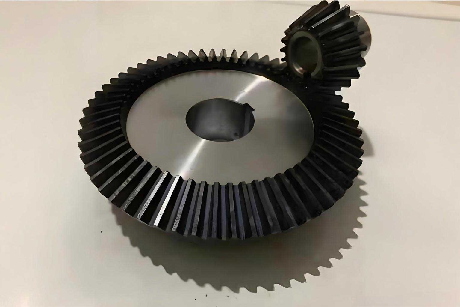
In this study, I focus on the design, manufacturing, dynamic analysis, and experimental validation of triangular end relief for double helical gears used in marine transmission systems. The motivation is straightforward: double helical gears carry large loads, balance axial forces, and operate with high power density, but they remain a major source of vibration and noise. I develop a multi-objective optimization method for triangular end relief, propose a three-section grinding wheel form grinding principle, and verify the vibration reduction effect through loaded transmission error tests and box vibration tests. Although my main object is the double helical gear, the same design logic can be adapted to miter gears when they require controlled contact impact, and I therefore keep the broader family of miter gears in view throughout the discussion.
1. Introduction
Involute gears are widely used in modern machinery because they transmit motion between arbitrary shafts with stable ratios and high efficiency. Planar gear mechanisms, including spur gears, helical gears, and double helical gears, are especially common for parallel-axis transmission. Spur gears tend to produce meshing impact and poor smoothness. Helical gears reduce impact but generate axial force. Double helical gears consist of two opposite-handed helical gear sets, so the axial forces from the left and right sides cancel each other. This makes double helical gears compact, highly loadable, and suitable for high-speed and heavy-load marine applications. I note that miter gears, which usually transmit motion between intersecting axes, have a different kinematic geometry, but they also benefit from tooth flank modification when impact and noise must be controlled.
With the rapid development of marine vessels, the acoustic stealth performance of transmission systems has become more demanding. A double helical gear pair is excited not only by external loads but also by internal excitations such as time-varying meshing stiffness and meshing impact force. These excitations travel through bearings and the gearbox housing, producing vibration and noise. Excessive vibration shortens service life and increases the risk of detection. Therefore, reducing vibration and noise through tooth surface modification is an important research direction. Compared with conventional profile modification and lead modification, triangular end relief is a newer approach. It modifies only the tooth root and tooth tip regions along a diagonal direction, while the middle working region remains almost unchanged. This preserves a large effective contact area, reduces meshing impact force, and lowers loaded transmission error fluctuation. I also consider that miter gears under similar high-load conditions can use the same conceptual strategy after suitable coordinate transformation.
Prior studies on triangular end relief have addressed modification amount calculation, modification curve selection, and manufacturing methods such as shaving and grinding. However, the efficiency and accuracy of some traditional methods remain limited. For double helical gears in marine applications, high-precision hard tooth surface grinding is required. Form grinding, which uses a line contact between the grinding wheel and the tooth surface, offers higher efficiency than generating grinding. With advances in CNC technology, servo control, and wheel dressing, form grinding can achieve high accuracy and efficiency. This motivates me to combine triangular end relief design with three-section grinding wheel form grinding for double helical gears. The same principle can later be extended to miter gears when their tooth flank geometry is properly parameterized.
2. Tooth Surface Design and Optimization
2.1 Standard Tooth Surface
I establish a coordinate system in which an imaginary generating rack cutter generates one side of the double helical gear. The left-handed imaginary rack cutter is used to generate the right-handed tooth side, and the opposite side is obtained by symmetric mapping about the mid-plane of the relief groove. For the standard involute helical surface, the position vector, unit normal vector, and meshing equation in the workpiece coordinate system are written as follows:
$$
\mathbf{r}_{ti}(u_i,l_i,\theta_i)=\mathbf{M}_{i,ti}\mathbf{r}_{ti},
$$
$$
\mathbf{n}_{ti}(u_i,l_i,\theta_i)=\mathbf{L}_{i,ti}\mathbf{n}_{ti},
$$
$$
f_i(u_i,l_i,\theta_i)=\mathbf{n}_{ti}\cdot\frac{\partial\mathbf{r}_{ti}}{\partial\theta_i}=0.
$$
Here, the subscript $$i=1,2$$ denotes the pinion and the gear, respectively. The parameters $$u_i$$ and $$l_i$$ describe the rack cutter surface, and $$\theta_i$$ is the workpiece rotation angle. For the root fillet generated by the rack cutter tip, I use a separate transition surface:
$$
\mathbf{r}’_i(\phi_i,l_i,\theta_i)=\mathbf{M}_{i,ti}\mathbf{r}’_{ti},
$$
$$
\mathbf{n}’_i(\phi_i,l_i,\theta_i)=\mathbf{L}_{i,ti}\mathbf{n}’_{ti},
$$
$$
f’_i(\phi_i,l_i,\theta_i)=\mathbf{n}’_{ti}\cdot\frac{\partial\mathbf{r}’_{ti}}{\partial\theta_i}=0.
$$
The basic parameters of the double helical gear pair used in my study are listed in Table 1. The pinion has 30 teeth, the gear has 72 teeth, the normal module is 5 mm, the pressure angle is 20 degrees, and the helix angle is 33.273 degrees. The pinion is left-right handed, and the gear is right-left handed. The working speed is 2500 r/min for the vibration test, and the rated load is 3000 Nm. I use these parameters consistently in the design, optimization, grinding, dynamic analysis, and experiments.
| Parameter | Pinion | Gear |
|---|---|---|
| Number of teeth | 30 | 72 |
| Normal module (mm) | 5 | |
| Pressure angle (deg) | 20 | |
| Helix angle (deg) | 33.273 | |
| Handedness | left-right | right-left |
| Face width (mm) | 44 x 2 | 40 x 2 |
| Relief groove (mm) | 46 | 50 |
| Speed (r/min) | 2500 | — |
| Rated torque (Nm) | — | 3000 |
2.2 Triangular End Relief Surface
Triangular end relief is defined according to ISO 21771. I treat the tooth tip and tooth root modification regions separately. The starting lines of modification on the rotating projection plane are determined by the instantaneous contact lines corresponding to the tip and root modification heights. For a point $$P$$ inside the modification region, the modification amount is
$$
\delta(z,x’)=
\begin{cases}
C_{Ea}\left(\frac{l_p}{l_a}\right)^{k_a}, & P\in ABC,\\[6pt]
C_{Ef}\left(\frac{l_p}{l_f}\right)^{k_f}, & P\in DEF,\\[6pt]
0, & \text{otherwise}.
\end{cases}
$$
Here, $$C_{Ea}$$ and $$C_{Ef}$$ are the maximum modification amounts at the tip and root, $$l_a$$ and $$l_f$$ are the modification lengths, $$l_p$$ is the distance from point $$P$$ to the corresponding starting line, and $$k_a$$ and $$k_f$$ are the curve orders. When $$k_a=k_f=1$$, the modification curve is linear. When $$k_a=k_f=2$$, the modification curve is a quadratic parabola. I consider both types because linear triangular end relief is easier to manufacture, while quadratic parabolic triangular end relief can provide smoother transition and better dynamic behavior. The same mathematical form can be used for miter gears if their projection plane and contact line are redefined.
The modified tooth surface is obtained by superimposing the modification amount on the standard working tooth surface along its normal direction:
$$
\mathbf{r}_{1m}(u_1,l_1,\theta_1)=\mathbf{r}_1(u_1,l_1,\theta_1)+\delta(z,x’)\mathbf{n}_1(u_1,l_1,\theta_1),
$$
$$
\mathbf{n}_{1m}(u_1,l_1,\theta_1)=
\mathbf{n}_1(u_1,l_1,\theta_1)+
\delta(z,x’)\left(
\frac{\partial\mathbf{n}_1}{\partial u_1}+
\frac{\partial\mathbf{n}_1}{\partial l_1}
\right).
$$
I apply triangular end relief only to the pinion. The gear remains a standard involute double helical gear. This choice reduces manufacturing complexity and keeps the gear pair interchangeable. The modification region includes the tooth tip near the relief groove and the tooth root near the outer ends for one tooth side, and the opposite arrangement for the other tooth side. This creates the diagonal, triangular pattern that gives the method its name.
2.3 Tooth Contact Analysis and Loaded Tooth Contact Analysis
I use tooth contact analysis, abbreviated as TCA, to calculate the geometric contact path, transmission error, and contact pattern. For a double helical gear pair, the contact analysis can be treated as two equivalent helical gear pairs. The two continuous tangent surfaces must have a common contact point and a common normal in the fixed coordinate system. The TCA equations are
$$
\mathbf{r}_f^{(1)}(u_1,l_1,\epsilon,\theta_1)=\mathbf{r}_f^{(2)}(u_2,l_2,\theta_2),
$$
$$
\mathbf{n}_f^{(1)}(u_1,l_1,\epsilon,\theta_1)=\mathbf{n}_f^{(2)}(u_2,l_2,\theta_2).
$$
Here, $$\epsilon$$ is the axial floating displacement of the pinion. After solving these equations, I obtain the geometric transmission error and the contact imprint. Then I use loaded tooth contact analysis, abbreviated as LTCA, to solve the load distribution and loaded transmission error. I generate a finite element mesh for the pinion and gear, compute the normal flexibility matrix, and superimpose the flexibility matrices of the two bodies. The contact points are discretized along the major axis of the contact ellipse. For four possible contacting tooth pairs, denoted by I, II, III, and IV, the initial gap before deformation is
$$
\mathbf{w}_k=\mathbf{\delta}_k+\mathbf{b}_k,\quad k=\mathrm{I},\mathrm{II},\mathrm{III},\mathrm{IV}.
$$
After deformation under load $$P_0$$, the displacement coordination equation is
$$
\mathbf{F}_k\mathbf{p}_k+\mathbf{w}_k=\mathbf{Z}_k+\mathbf{d}_k,\quad k=\mathrm{I},\mathrm{II},\mathrm{III},\mathrm{IV}.
$$
The force balance condition is
$$
\sum_{j=1}^{n}p_j^{\mathrm{I}}+
\sum_{j=1}^{n}p_j^{\mathrm{II}}+
\sum_{j=1}^{n}p_j^{\mathrm{III}}+
\sum_{j=1}^{n}p_j^{\mathrm{IV}}=P_0.
$$
For a double helical gear pair, the axial forces from the left and right sides must balance because the pinion floats axially. Therefore, I add the following constraint:
$$
\sum_{j=1}^{n}p_j^{\mathrm{I}}\cos\eta_j+
\sum_{j=1}^{n}p_j^{\mathrm{II}}\cos\eta_j
=
\sum_{j=1}^{n}p_j^{\mathrm{III}}\cos\eta_j+
\sum_{j=1}^{n}p_j^{\mathrm{IV}}\cos\eta_j.
$$
The LTCA problem is solved as a mathematical programming problem:
$$
\min \frac{1}{2}\mathbf{p}^T\mathbf{F}\mathbf{p}+\mathbf{p}^T(\mathbf{Z}+\mathbf{w}),
$$
$$
\text{subject to } \mathbf{e}^T\mathbf{p}=P_0,\quad \mathbf{p}\ge0,\quad \mathbf{d}\ge0,\quad \mathbf{p}^T\mathbf{d}=0.
$$
After solving, I obtain the normal displacement $$\mathbf{Z}$$, the discrete load $$\mathbf{p}$$, and the normal gap $$\mathbf{d}$$. The load sharing coefficient of a contact position is
$$
L_k=\frac{\sum_{j=1}^{n}p_{jk}}{P_0},\quad k=\mathrm{I},\mathrm{II},\mathrm{III},\mathrm{IV}.
$$
The loaded transmission error is calculated from the normal displacement as
$$
T_e=\frac{3600\times180}{\pi}\frac{Z}{r_b\cos\beta}.
$$
The fluctuation of the loaded transmission error is defined as
$$
\Delta T_e=\max(T_e)-\min(T_e).
$$
This fluctuation is a key excitation for vibration and noise. A smaller $$\Delta T_e$$ generally means lower dynamic excitation. I therefore use it as one of the optimization objectives.
2.4 Meshing Impact Force
The meshing impact force is caused by the deviation of the actual meshing point from the ideal meshing point due to manufacturing error, installation error, and tooth deformation. Under load, the previous tooth pair deforms, producing a base pitch difference. The next tooth pair then contacts prematurely, causing meshing interference. For a standard involute surface, the actual contact point can be found by rotating the gear back by an angle $$\Delta\varphi_{k2}$$ and solving the geometric relations. For a modified surface, the interference may be avoided under small load, but a slight deviation from the ideal path still occurs. I calculate the actual impact point using TCA and LTCA, and then compute the relative velocity at that point:
$$
\mathbf{v}_{12}^{f}=
\left(\mathbf{w}^{(1)}_f-\mathbf{w}^{(2)}_f\right)\times\mathbf{r}^{(1)}_f
–
\mathbf{w}^{(2)}_f\times\mathbf{E}_f.
$$
The impact kinetic energy is
$$
E_k=\frac{1}{2}\frac{J_1J_2}{J_1r_{b2}^2+J_2r_{b1}^2}\left(v_{12}^{f}\right)^2.
$$
The maximum impact force is
$$
F_s=
\sqrt{
k_s\frac{J_1J_2}{J_1r_{b2}^2+J_2r_{b1}^2}
}
v_{12}^{f}.
$$
Here, $$k_s$$ is the meshing stiffness at the actual impact point, obtained from LTCA. The impact force is the second optimization objective. I note that for miter gears, the same energy method can be used, but the relative velocity and contact point must be expressed in the miter gear coordinate system.
2.5 Multi-Objective Optimization Model
I formulate the triangular end relief optimization as a multi-objective problem. The objectives are to minimize the loaded transmission error fluctuation and the meshing impact force. The design variables are the tip maximum modification amount, tip modification height, root maximum modification amount, and root modification height:
$$
\min Q=
w_1\frac{\Delta T_e}{\Delta T_{e0}}+
w_2\frac{F_s}{F_{s0}},
$$
$$
\Delta T_e=\max(T_e)-\min(T_e),
$$
$$
\text{subject to } Q_{\min}\le y_1\le Q_{\max},\quad
h_{a\min}\le y_2\le h_{a\max},\quad
Q_{\min}\le y_3\le Q_{\max},\quad
h_{f\min}\le y_4\le h_{f\max}.
$$
Here, $$\Delta T_{e0}$$ and $$F_{s0}$$ are the loaded transmission error fluctuation and meshing impact force of the standard tooth surface. The weights $$w_1$$ and $$w_2$$ are both set to 0.5. The optimization ranges are determined from the single-tooth and double-tooth contact boundaries, the pitch circle, the tip modification termination line, and the root modification termination line. I use the NSGA-II genetic algorithm because it can handle non-analytical objective functions, multiple local optima, and discrete design variables. The population size is 200, and the number of generations is 400. The crossover probability is 0.8, and the mutation probability is 0.2.
| Optimization variable | Range | Linear value | Quadratic value |
|---|---|---|---|
| Tip maximum modification amount (micrometer) | 8 to 20 | 16.10 | 16.53 |
| Tip modification height (mm) | 2.01 to 5.00 | 2.72 | 4.52 |
| Root maximum modification amount (micrometer) | 8 to 20 | 9.31 | 11.63 |
| Root modification height (mm) | 1.27 to 4.04 | 2.81 | 2.44 |
2.6 Optimization Results
For the linear triangular end relief, the objective function stabilizes at about the 43rd generation, and the minimum value is 0.15. For the quadratic parabolic triangular end relief, the objective function stabilizes at about the 50th generation, and the minimum value is 0.11. The optimized parameters are listed in Table 2. The quadratic type achieves a lower objective value, which indicates a better compromise between loaded transmission error fluctuation and meshing impact force. I also observe that the modification surfaces follow the intended triangular pattern. For one tooth side, the root modification is near the outer ends and the tip modification is near the relief groove. For the opposite tooth side, the arrangement is reversed.
| Case | Loaded transmission error fluctuation (arcsec) | Reduction relative to standard | Meshing impact force (N) | Reduction relative to standard |
|---|---|---|---|---|
| Standard involute | 0.8102 | — | 2983 | — |
| Linear triangular end relief | 0.1973 | 75.55% | 191 | 93.60% |
| Quadratic parabolic triangular end relief | 0.1319 | 83.70% | 168 | 94.37% |
The contact pattern of the standard tooth surface shows edge contact at the beginning and end of meshing. The maximum load sharing coefficient is 0.3378. After linear triangular end relief, the load sharing coefficient in the modification region decreases, and the maximum value becomes 0.36. After quadratic parabolic triangular end relief, the maximum load sharing coefficient is 0.3585. Although the maximum load sharing coefficient increases slightly, the loaded transmission error fluctuation and impact force drop dramatically. This is because the diagonal modification along the contact line compensates for the loaded deformation and reduces the abrupt change of meshing stiffness. I also note that the multi-load variation trend of the loaded transmission error fluctuation and the impact force are similar. The minimum values appear near the design load of 3000 Nm. This confirms that the triangular end relief is load-dependent and should be optimized for the intended working condition. The same load-dependent behavior should be expected for miter gears if they are modified in a similar way.
3. Three-Section Grinding Wheel Form Grinding
3.1 Coordinate Transformation from Workpiece to Grinding Wheel
To manufacture the optimized triangular end relief, I propose a three-section grinding wheel form grinding method. The basic idea is that the linear triangular end relief surface can be approximated by three helical surfaces with different basic parameters. The tip modification is realized by increasing the normal pressure angle or decreasing the normal module, and the root modification is realized by decreasing the normal pressure angle or increasing the normal module. The lead modification is realized by changing the helix angle. For the quadratic parabolic triangular end relief, I add a quadratic parabolic profile modification on top of the linear three-section method. I establish the coordinate transformation from the workpiece to the grinding wheel as follows:
$$
\mathbf{r}_t=\mathbf{M}_{t1}(\gamma_m,E_t,L_t)\mathbf{r}_1,
$$
$$
\mathbf{n}_t=\mathbf{L}_{t1}(\gamma_m,E_t,L_t)\mathbf{n}_1.
$$
Here, $$\gamma_m$$ is the wheel setting angle, $$E_t$$ is the center distance between the wheel and the workpiece, and $$L_t$$ is the axial movement of the wheel. Since the grinding wheel is a surface of revolution, the normal vector at any point on the wheel surface must intersect or be parallel to the wheel axis. The contact condition is
$$
f_t(u_1,l_1,\theta_1)=
\mathbf{n}_t(u_1,l_1,\theta_1)\cdot
\left(\mathbf{z}_t\times\mathbf{r}_t(u_1,l_1,\theta_1)\right)=0.
$$
By solving this equation at a fixed workpiece rotation angle, I obtain the contact line between the wheel and the tooth surface. The wheel profile is then obtained by rotating the contact points into the wheel axial plane:
$$
y_c=\sqrt{y_t^2+z_t^2},\quad x_c=x_t.
$$
3.2 CNC Form Grinding Machine Settings
I model a five-axis CNC form grinding machine with two linear axes and three rotary axes. The main motions are the high-speed rotation of the grinding wheel spindle, the radial feed of the wheel carriage relative to the workpiece spindle, the indexing rotation of the workpiece spindle, the axial movement of the workpiece table, and the wheel swivel for the helix angle. After comparing the virtual machine coordinate system and the real machine coordinate system, I obtain the machine axis parameters as
$$
\psi_a=\theta_1,\quad
\psi_b=\gamma_m,\quad
C_x=-L_t,\quad
C_y=E_t.
$$
For the double helical pinion in Table 1, with a grinding wheel diameter of 100 mm, the machine settings are given in Table 3. These settings are used to control the CNC axes and to dress the grinding wheel. The same procedure can be applied to miter gears if the coordinate transformation and wheel profile equations are rewritten for intersecting axes.
| Setting | Value |
|---|---|
| Axial movement $$C_x$$ | $$-136.7044\theta_1$$ |
| Radial movement $$C_y$$ | 139.7058 |
| Workpiece rotation $$\psi_a$$ | $$\theta_1$$ |
| Wheel swivel $$\psi_b$$ | 0.5807 rad |
3.3 Optimization of the Three-Section Grinding Wheel
I define the target modified tooth surface for the tip and root regions. The actual surface generated by the three-section wheel is compared with the target surface at a set of discrete points. The normal deviation at point $$i$$ for region $$j$$ is
$$
h_{i,j}^{t}(d_j^t)=
\left(\mathbf{p}_{i,j}^{t}-\mathbf{p}_{i,j}^{*,t}\right)\cdot
\mathbf{n}_{i,j}^{t}.
$$
The optimization objective is to minimize the sum of squares of the normal deviations:
$$
\min f_j(\mathbf{d}_j^t)=
\mathbf{H}_j^T(\mathbf{d}_j^t)\mathbf{H}_j(\mathbf{d}_j^t),
$$
$$
\mathbf{H}_j(\mathbf{d}_j^t)=
\left[h_{1,j}^t,h_{2,j}^t,\ldots,h_{k,j}^t\right]^T.
$$
For the linear triangular end relief, the design variables are
$$
\mathbf{d}_1=
\left[m_n,\alpha_n,\beta\right]^T.
$$
For the quadratic parabolic triangular end relief, the design variables are
$$
\mathbf{d}_2=
\left[m_n,\alpha_n,\beta,h,\varsigma\right]^T,
$$
where $$h$$ is the profile modification height and $$\varsigma$$ is the profile modification amount. I use NSGA-II again with a population of 200 and 400 generations. The optimized parameters are listed in Table 4 and Table 5. For the linear case, the maximum tooth surface deviation is less than 1 micrometer. For the quadratic case, the maximum deviation is less than 3 micrometers. The slightly larger deviation in the quadratic case comes from the additional parabolic profile approximation and the interaction between the three basic helical surfaces.
| Region | Module (mm) | Pressure angle (deg) | Helix angle (deg) | Deviation square sum |
|---|---|---|---|---|
| Tip | 5.00053 | 20.5342 | 33.4012 | $$6.12\times10^{-7}$$ |
| Root | 5.00383 | 19.9219 | 33.2534 | $$1.30\times10^{-6}$$ |
| Region | Module (mm) | Pressure angle (deg) | Helix angle (deg) | Profile height (mm) | Profile amount (micrometer) | Deviation square sum |
|---|---|---|---|---|---|---|
| Tip | 4.9995 | 20.0423 | 33.3354 | 6.44 | 16.25 | $$1.12\times10^{-4}$$ |
| Root | 5.00432 | 19.9641 | 33.2498 | 3.89 | 3.50 | $$5.43\times10^{-5}$$ |
3.4 Manufacturing and Inspection
I manufactured the linear triangular end relief pinion on a CNC form grinding machine. The pinion is an integral shaft design, and I used double centers as the unified datum to improve positioning accuracy. The center holes were re-ground before grinding. The grinding wheel diameter was selected as 100 mm to avoid interference with the opposite tooth side and to leave enough clearance for wheel withdrawal. The grinding process had three steps. First, I used the standard wheel profile to grind all tooth surfaces. Second, I dressed the wheel to the root modification profile and ground the root modification region. Third, I dressed the wheel to the tip modification profile and ground the tip modification region.
I measured the tooth surface on a precision gear measuring instrument. The accuracy grade of the gear pair is grade 4 according to the relevant standard. The specified deviations are: total profile deviation 7.5 micrometers, total helix deviation 7.5 micrometers, single pitch deviation 5.0 micrometers, and total cumulative pitch deviation 18.0 micrometers. I planned three profile paths and three helix paths on each tooth side. The profile paths were at the root modification termination line, the pitch circle, and a point near the tip modification termination line. The helix paths were at 2 mm, 22 mm, and 42 mm along the face width. The measurement results are summarized in Table 6. Most deviations are within grade 4. One tip modification region on the left-handed tooth side exceeds the profile tolerance band by about 2 micrometers. The main causes are machine motion error, thermal effects, repeated positioning error of the spindle, and the difficulty of maintaining identical tool setting for the standard, tip, and root grinding steps. After several trial grinding, adjustment, and inspection cycles, the tooth profile, helix, and pitch deviations generally reach grade 4. I also performed a rolling test with red lead powder. The triangular end relief regions appear bright and do not pick up red lead, which verifies that the modified regions are correctly manufactured. I did not perform experimental validation for the quadratic parabolic three-section wheel because the additional profile modification makes the wheel dressing more complex and the current process is not yet mature. However, the numerical results indicate that it is feasible. The same three-section concept can be extended to miter gears when their wheel profile and machine settings are derived for intersecting axes.
| Deviation item | Specified value (micrometer) | Measured value (micrometer) | Grade |
|---|---|---|---|
| Total profile deviation | 7.5 | Within 9.5 for one tip region; others within 7.5 | Mostly grade 4 |
| Total helix deviation | 7.5 | Within 9.5 for one region; others within 7.5 | Mostly grade 4 |
| Single pitch deviation | 5.0 | Maximum 3.1 | Grade 4 |
| Total cumulative pitch deviation | 18.0 | Maximum 8.6 | Grade 4 |
4. Dynamic Characteristics
4.1 Twelve-Degree-of-Freedom Model
I establish a twelve-degree-of-freedom dynamic model for the double helical gear pair supported by sliding bearings. The model includes bending, torsion, and axial motions. The generalized displacement vector is
$$
\mathbf{q}=
\left[
y_{p1},z_{p1},\theta_{p1},
y_{g1},z_{g1},\theta_{g1},
y_{p2},z_{p2},\theta_{p2},
y_{g2},z_{g2},\theta_{g2}
\right]^T.
$$
Here, the subscripts $$p1$$ and $$p2$$ denote the left and right sides of the pinion, and $$g1$$ and $$g2$$ denote the left and right sides of the gear. The dynamic equations are derived from Newton’s law. For the left side of the pinion, the equations are
$$
m_{p1}\ddot{y}_{p1}+c_{p1y}\dot{y}_{p1}+k_{p1y}y_{p1}=-F_{n1}\cos\beta_1,
$$
$$
m_{p1}\ddot{z}_{p1}+c_{p1z}\left(\dot{z}_{p1}-\dot{z}_{p2}\right)+
k_{p1z}\left(z_{p1}-z_{p2}\right)=-F_{n1}\sin\beta_1,
$$
$$
I_{p1}\ddot{\theta}_{p1}=
F_{n1}R_{bp}-T_{p1}+F_{s1}R_{bp}.
$$
For the left side of the gear, the equations are
$$
m_{g1}\ddot{y}_{g1}+c_{g1y}\dot{y}_{g1}+k_{g1y}y_{g1}=F_{n1}\cos\beta_1,
$$
$$
m_{g1}\ddot{z}_{g1}+c_{g1z}\dot{z}_{g1}+k_{g1z}z_{g1}
+c_{g12z}\left(\dot{z}_{g1}-\dot{z}_{g2}\right)
+k_{g12z}\left(z_{g1}-z_{g2}\right)
=F_{n1}\sin\beta_1,
$$
$$
I_{g1}\ddot{\theta}_{g1}=
F_{n1}R_{bg}-T_{g1}+F_{s1}R_{bg}.
$$
Similar equations hold for the right side. The normal dynamic meshing force is
$$
F_{n1}=
c_{m1}\left[
\dot{y}_{p1}-\dot{y}_{g1}
+R_{bp}\dot{\theta}_{p1}-R_{bg}\dot{\theta}_{g1}
+\left(\dot{z}_{p1}-\dot{z}_{g1}\right)\tan\beta_1
\right]
+
k_{m1}\left[
y_{p1}-y_{g1}
+R_{bp}\theta_{p1}-R_{bg}\theta_{g1}
+\left(z_{p1}-z_{g1}\right)\tan\beta_1
\right].
$$
Here, $$c_{m1}$$ and $$k_{m1}$$ are the meshing damping and time-varying meshing stiffness. The meshing damping is calculated from the equivalent mass and the relative damping ratio. I assume a relative damping ratio of 0.1. The axial floating displacement of the pinion is denoted by $$\epsilon_z$$. Because the pinion floats, the left and right axial forces balance each other. This is one of the main advantages of double helical gears over miter gears, which cannot self-balance axial force in the same way.
4.2 Excitations
The time-varying meshing stiffness is obtained from LTCA. The comprehensive meshing stiffness is
$$
K_m=\frac{F_n}{Z_k}.
$$
I fit the discrete stiffness values with Hermite interpolation and then expand the result into a Fourier series. The meshing impact force is obtained from the impact calculation in Section 2.4. I fit the impact force versus meshing time with a polynomial and expand it into a Fourier series. The sliding bearing oil film stiffness and damping are obtained from the Reynolds equation. The dimensionless Reynolds equation is
$$
\frac{\partial}{\partial\varphi}
\left(
H^3\frac{\partial p}{\partial\varphi}
\right)
+
\left(\frac{D}{L}\right)^2
\frac{\partial}{\partial z}
\left(
H^3\frac{\partial p}{\partial z}
\right)
=
6\cos\varphi\frac{\partial H}{\partial\varphi}
+
12\frac{\partial H}{\partial\tau}.
$$
The oil film stiffness and damping coefficients are the partial derivatives of the oil film force with respect to displacement and velocity:
$$
k_{xx}=\frac{\partial F_x}{\partial x},\quad
k_{xy}=\frac{\partial F_x}{\partial y},\quad
k_{yx}=\frac{\partial F_y}{\partial x},\quad
k_{yy}=\frac{\partial F_y}{\partial y},
$$
$$
c_{xx}=\frac{\partial F_x}{\partial\dot{x}},\quad
c_{xy}=\frac{\partial F_x}{\partial\dot{y}},\quad
c_{yx}=\frac{\partial F_y}{\partial\dot{x}},\quad
c_{yy}=\frac{\partial F_y}{\partial\dot{y}}.
$$
4.3 Dynamic Response Results
I compared the dynamic responses of three cases: the standard double helical gear pair, the linear triangular end relief pair, and the quadratic parabolic triangular end relief pair. The standard pair has a comprehensive meshing stiffness fluctuation of $$1.16\times10^8$$ N/m. The linear triangular end relief reduces this fluctuation to $$2.4\times10^7$$ N/m, a reduction of 79.31%. The quadratic parabolic triangular end relief reduces it to $$1.6\times10^7$$ N/m, a reduction of 86.20%. The meshing impact force is 2983 N for the standard pair, 191 N for the linear modification, and 168 N for the quadratic modification. The vibration acceleration along the meshing line is expressed as a root mean square value. The standard pair has 70.24 m/s2. The linear modification has 11.83 m/s2, a reduction of 83.15%. The quadratic modification has 8.43 m/s2, a reduction of 88%. The dynamic load fluctuation along the meshing line is 624 N for the standard pair, 206 N for the linear modification, and 161 N for the quadratic modification. These results are summarized in Table 7.
| Quantity | Standard | Linear triangular end relief | Quadratic triangular end relief |
|---|---|---|---|
| Meshing stiffness fluctuation (N/m) | $$1.16\times10^8$$ | $$2.4\times10^7$$ | $$1.6\times10^7$$ |
| Meshing impact force (N) | 2983 | 191 | 168 |
| Meshing line acceleration RMS (m/s2) | 70.24 | 11.83 | 8.43 |
| Dynamic load fluctuation (N) | 624 | 206 | 161 |
The frequency-domain response shows that the standard pair has a dominant peak at the third harmonic. The linear modification shifts the dominant peak to the first harmonic and reduces its amplitude. The quadratic modification also reduces the peak amplitude. The multi-load vibration acceleration follows the same trend as the loaded transmission error fluctuation and the impact force. It first decreases and then increases with load. The minimum vibration occurs near the design load of 3000 Nm. This confirms that the triangular end relief is effective over a range of loads and that the quadratic type provides better vibration reduction than the linear type. I also observe that the dynamic behavior of miter gears under similar loads would require a separate model because their axial force balance and contact geometry differ, but the excitation reduction mechanism remains comparable.
5. Experimental Validation
5.1 Test Objects and Conditions
I selected the linear triangular end relief for experimental validation because it is easier to manufacture than the quadratic type. The test gear pairs are a standard double helical pinion and gear pair, denoted as P01G01, and a linear triangular end relief pinion with a standard gear, denoted as P02G01. The basic parameters are the same as in Table 1. The pinion P02 uses the optimized linear modification parameters in Table 2. Both the pinion and the gear are grade 4. The loaded transmission error test is performed at a pinion speed of 4.18 r/min with gear torques of 1000, 1500, 2000, 2500, 3000, 3500, and 4000 Nm. The vibration test is performed at a pinion speed of 2500 r/min with gear torques of 1000, 2000, 3000, and 3600 Nm. The torque limit of the driving motor is 3600 Nm, so the highest vibration test load is 3600 Nm.
5.2 Loaded Transmission Error Measurement
The loaded transmission error measurement system consists of two high-precision encoders, a synchronous data acquisition card, an industrial computer, and custom processing software. The encoder accuracy is better than 0.1 arcsec. The measurement system accuracy is calibrated to be within 0.05 arcsec, which is sufficient for this study. I sample the transmission error for 30 seconds, which covers more than 50 meshing cycles. I remove the low-frequency shaft frequency component caused by cumulative pitch error using median filtering. The remaining tooth frequency component is used to calculate the loaded transmission error fluctuation. I repeat each measurement three times and take the average. The loaded transmission error is calculated as
$$
\text{LTTE fluctuation}=\max(T_e)-\min(T_e).
$$
5.3 Loaded Transmission Error Results
The measured loaded transmission error fluctuations for P01G01 and P02G01 under multiple loads are listed in Table 8. The simulated values are also listed for comparison. At the design load of 3000 Nm, the measured loaded transmission error fluctuation of P02G01 is 0.76 arcsec, while that of P01G01 is 1.16 arcsec. This is a reduction of 34%. The simulated values are 0.20 arcsec for P02G01 and 0.81 arcsec for P01G01, a reduction of 75%. The measured values are generally higher than the simulated values because manufacturing errors, assembly errors, and housing errors are not included in the simulation. The difference is about 30% for the standard pair and about 60% for the modified pair. The larger difference for the modified pair is due to the fact that the three-section form grinding process is still being developed and the manufacturing accuracy of the triangular end relief is more difficult to control. The measured minimum loaded transmission error fluctuation for P02G01 occurs at 2500 Nm rather than at the design load of 3000 Nm. This shift is caused by the combined effect of manufacturing error, housing error, and installation error. Nevertheless, the experimental results confirm that the linear triangular end relief reduces the loaded transmission error fluctuation under multiple loads. The trend of the measured values agrees with the simulated values. This validates the optimization design method. I also note that for miter gears, the same measurement principle can be applied, but the encoder mounting and coordinate alignment must be adapted to the intersecting shaft arrangement.
| Load (Nm) | 1000 | 1500 | 2000 | 2500 | 3000 | 3500 | 4000 |
|---|---|---|---|---|---|---|---|
| P01G01 measured (arcsec) | 0.73 | 0.80 | 0.86 | 1.02 | 1.16 | 1.25 | 1.33 |
| P01G01 simulated (arcsec) | 0.26 | 0.39 | 0.53 | 0.67 | 0.81 | 0.95 | 1.09 |
| P02G01 measured (arcsec) | 0.91 | 0.85 | 0.74 | 0.69 | 0.76 | 0.86 | 1.01 |
| P02G01 simulated (arcsec) | 0.48 | 0.45 | 0.36 | 0.27 | 0.20 | 0.26 | 0.36 |
5.4 Vibration Results
The vibration test is conducted on a mechanically closed test rig. The gearbox is supported by sliding bearings. I install a three-axis accelerometer at the bottom foot of the gearbox. The vertical direction is taken as the main vibration direction because it represents the overall vibration response. I sample the vibration signal at 51200 Hz. At a pinion speed of 2500 r/min, each meshing period contains more than 40 sampling points, which is sufficient to capture the waveform. I take 100 meshing periods and calculate the root mean square value. I repeat each measurement three times and take the average. The measured vibration acceleration results are listed in Table 9. At 3000 Nm, the measured vibration acceleration of P02G01 is 3.36 m/s2, while that of P01G01 is 4.22 m/s2. This is a reduction of 20%. The simulated meshing line acceleration is 11.83 m/s2 for P02G01 and 70.24 m/s2 for P01G01, a reduction of 83%. The measured vibration is much smaller than the simulated meshing line acceleration because the sliding bearing oil film and the gearbox housing provide significant damping. The trend of the measured vibration with load is similar to that of the loaded transmission error fluctuation. A larger loaded transmission error fluctuation corresponds to a larger box foot vibration. The multi-load measured vibration of P02G01 is lower than that of P01G01, and the trend of the measured and simulated results is similar. This confirms that the linear triangular end relief reduces the vibration of the double helical gear pair. I also consider that miter gears in a similar test rig would show a comparable response if the modification and bearing support are properly designed.
| Load (Nm) | 1000 | 2000 | 3000 | 3600 |
|---|---|---|---|---|
| P01G01 measured box foot acceleration (m/s2) | 3.34 | 3.51 | 4.22 | 4.76 |
| P01G01 simulated meshing line acceleration (m/s2) | 22.72 | 44.55 | 70.24 | 80.12 |
| P02G01 measured box foot acceleration (m/s2) | 2.93 | 2.33 | 3.36 | 4.07 |
| P02G01 simulated meshing line acceleration (m/s2) | 26.87 | 20.21 | 11.83 | 14.86 |
6. Conclusions
I have studied the design, manufacturing, dynamic behavior, and experimental validation of triangular end relief for double helical gears. The main conclusions are as follows.
First, I derived the standard tooth surface equation and the triangular end relief tooth surface equation for double helical gears. The modification surface is obtained by superimposing the modification amount on the standard involute surface along its normal direction. I designed both linear and quadratic parabolic modification curves. The quadratic parabolic triangular end relief provides a smoother transition and better optimization results than the linear type. Under the rated load of 3000 Nm, the linear type reduces the loaded transmission error fluctuation by 75.55% and the meshing impact force by 93.60% relative to the standard tooth surface. The quadratic type reduces them by 83.70% and 94.37%, respectively. These results demonstrate the effectiveness of the multi-objective optimization method. I also note that the same optimization framework can be applied to miter gears after proper coordinate transformation and contact analysis.
Second, I proposed a three-section grinding wheel form grinding method to realize triangular end relief. The linear triangular end relief is approximated by three helical surfaces with different modules, pressure angles, and helix angles. The quadratic parabolic triangular end relief is realized by adding a quadratic profile modification to the linear three-section method. I derived the coordinate transformation, wheel profile equation, and CNC machine axis parameters. The optimized maximum tooth surface deviation is less than 1 micrometer for the linear type and less than 3 micrometers for the quadratic type. The linear triangular end relief pinion was successfully manufactured. The measured tooth profile, helix, and pitch deviations generally reach grade 4. The rolling test confirms that the modification regions are correctly formed. The current process still requires several trial grinding and adjustment cycles. For the quadratic type, the wheel dressing is more complex, and the process is not yet mature enough for experimental validation. However, the numerical results show that it is feasible. In future work, I plan to improve the wheel dressing and machine adjustment to reduce the deviation. The same three-section method can be adapted to miter gears if their generating geometry and wheel profile are properly derived.
Third, I established a twelve-degree-of-freedom dynamic model for the double helical gear pair supported by sliding bearings. The model includes bending, torsion, and axial motions. I calculated the time-varying meshing stiffness from LTCA and the meshing impact force from the energy method. I also calculated the sliding bearing oil film stiffness and damping from the Reynolds equation. The dynamic results show that the triangular end relief reduces the meshing stiffness fluctuation, the impact force, and the meshing line acceleration. The quadratic type performs better than the linear type. The multi-load vibration acceleration follows the same trend as the loaded transmission error fluctuation and the impact force. The minimum vibration occurs near the design load.
Fourth, I built a loaded transmission error test rig and a mechanically closed vibration test rig. The loaded transmission error measurement system has an accuracy better than 0.05 arcsec. The vibration measurement system uses a three-axis accelerometer and a high-speed data acquisition system. The experimental results show that the loaded transmission error fluctuation of the linear triangular end relief pair is lower than that of the standard pair under multiple loads. The box foot vibration acceleration follows the same trend as the loaded transmission error fluctuation. At 3000 Nm, the measured loaded transmission error fluctuation is reduced by 34%, and the measured box foot vibration acceleration is reduced by 20%. The measured and simulated trends agree well, although the measured values are higher than the simulated values because of manufacturing and assembly errors. The minimum vibration load deviates from the design load due to these errors. Overall, the experiments confirm that linear triangular end relief can reduce the vibration and noise of double helical gear pairs. I also consider that miter gears could benefit from a similar design if their specific geometry and operating conditions are taken into account.
For future work, I plan to extend the method in three directions. First, I will improve the three-section grinding wheel process for quadratic parabolic triangular end relief by using more sophisticated wheel dressing and compensation strategies. Second, I will include manufacturing errors in the optimization model so that the simulated results can better match the experimental results. Third, I will build a three-dimensional finite element model of the double helical gear, sliding bearing, and gearbox housing to predict the box foot vibration directly. I will also extend the method to miter gears, because although miter gears and double helical gears have different axis arrangements, both require precise tooth surface design to reduce impact and noise. The triangular end relief concept, the multi-objective optimization method, and the three-section form grinding principle provide a useful foundation for such an extension.