
I treat the pressure angle of straight bevel gears as one of the most sensitive internal parameters in the entire manufacturing chain. In my experience, even when the outer geometry of a straight bevel gear appears correct, small deviations in the local pressure angle can change the contact pattern, the transmission error, the load distribution, and the vibration signature. For straight bevel gears, the pressure angle is not merely a nominal design number; it is a distributed property of the tooth flank. If I measure only one or two points on a flank, I cannot reconstruct the pressure angle with enough confidence. Therefore, I use a three-dimensional coordinate measuring instrument, a spherical probe, a parametric tooth-flank model, and a least-squares estimation procedure to extract the pressure angle error of straight bevel gears.
My main purpose here is to describe a measurement and computation method that I can apply directly to production straight bevel gears. I first represent the tooth surface of straight bevel gears with a mathematical model. I then relate the model to the coordinate system of the measuring instrument. After that, I measure multiple points on the left and right flanks. Finally, I estimate the pressure angle and its error by least-squares fitting. The method gives me a practical way to correct machining parameters and to improve the accuracy of straight bevel gears.
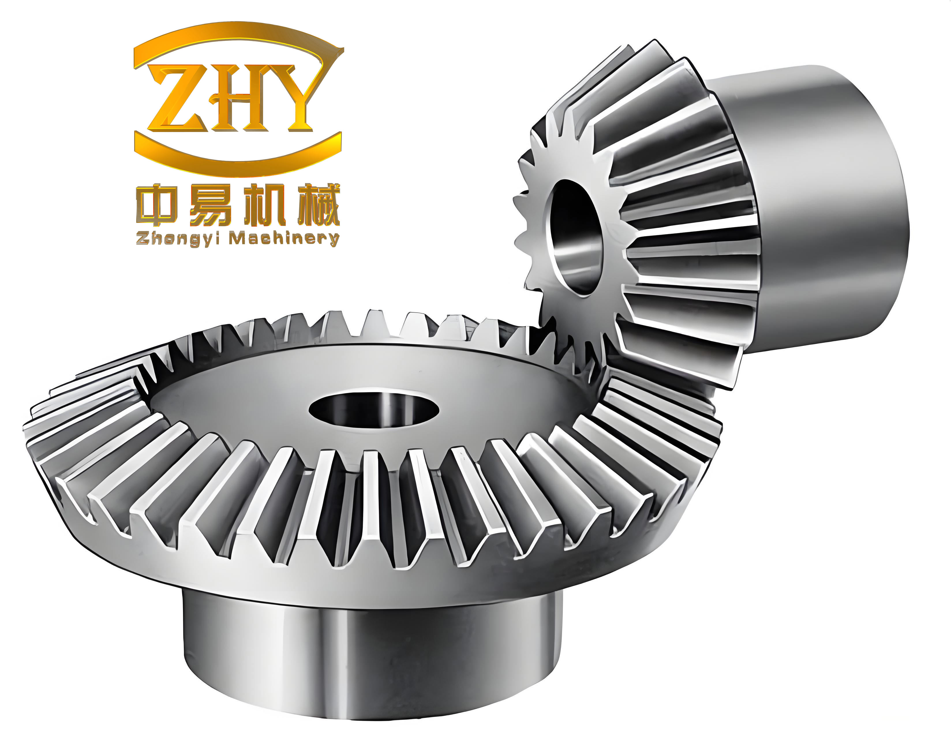
1. Why I Focus on Pressure Angle Error in Straight Bevel Gears
Straight bevel gears can be produced by milling, slotting, hobbing, casting, and other processes. Each process has its own kinematic errors, tool limitations, fixture errors, thermal drift, and dynamic effects. These factors do not affect every point of the tooth surface in the same way. In many cases, the deviation appears as a local change in the effective pressure angle. When the pressure angle error becomes large, the tooth profile of straight bevel gears no longer follows the intended involute-like form, and the transmission becomes less stable. I have seen that repeated trial cuts are often used to compensate for this problem, but trial cuts are expensive and not always deterministic.
The pressure angle is a fundamental calculation parameter of straight bevel gears. In manufacturing, I want to know whether the pressure angle at each point of the tooth flank is accurate. That accuracy is directly connected to the machining precision and the transmission stability of straight bevel gears. My method uses a three-dimensional coordinate measuring instrument to obtain multiple point coordinates on the tooth surface. Then, through least-squares analysis, I extract the pressure angle error. The result can be fed back into the machining process so that the tool setting, the generating motion, and the machine parameters can be corrected.
2. Nomenclature and Main Symbols
| Symbol | Meaning in my model |
|---|---|
| $$\alpha$$ | The pressure angle of the straight bevel gear tooth flank |
| $$\alpha_0$$ | The theoretical or design pressure angle |
| $$\Delta\alpha$$ | The pressure angle error, defined as $$\alpha-\alpha_0$$ |
| $$\Delta$$ | The tooth-trace offset or tooth-direction error |
| $$u,v$$ | Parameters that describe a point on the generating tooth surface |
| $$\phi$$ | The rotation angle of the generating crown gear |
| $$\Phi$$ | The angular offset between the gear coordinate system and the measuring coordinate system |
| $$\varepsilon$$ | The back-cone error of the straight bevel gear |
| $$r_0$$ | The radius of the spherical probe |
| $$\mathbf{X}$$ | A position vector on the tooth surface |
| $$\mathbf{N}$$ | A unit normal vector of the tooth surface |
| $$\mathbf{M}$$ | The center coordinate of the spherical probe |
| $$\mathbf{W}$$ | The relative velocity between the tool and the workpiece |
| $$z$$ | The number of teeth of a straight bevel gear |
| $$m$$ | The module of the straight bevel gears |
| $$R$$ | The back-cone distance |
| $$t$$ | A conformity or residual indicator of the coordinate measurements |
I use these symbols consistently. When I refer to straight bevel gears, I keep the same parametric surface description for both the left and right flanks. The sign of the pressure angle is treated according to the flank side and the chosen normal direction.
3. Mathematical Representation of the Tooth Surface of Straight Bevel Gears
I begin with a standard imaginary crown gear. The cutting edge surface of this crown gear is the generating surface for straight bevel gears. In the coordinate system $$O-xyz$$, I let $$\alpha$$ be the pressure angle of the generating surface and let $$\Delta$$ be the tooth-direction offset. I introduce two surface parameters $$u$$ and $$v$$. A point on the generating tooth surface can be written in a compact parametric form.
One convenient representation is
$$
\mathbf{x}(u,v)=
\begin{bmatrix}
u\sin\alpha+\Delta\cos\alpha\\
v\\
u\cos\alpha-\Delta\sin\alpha
\end{bmatrix}.
$$
In this expression, $$u$$ controls the position along the tooth profile direction, and $$v$$ controls the position along the tooth trace direction. The term $$\Delta$$ shifts the surface along the tooth direction. Since $$\Delta$$ is usually small, its effect is subtle but measurable in the coordinate data.
I also define the normal direction of the generating surface. For the same parameterization, the unit normal can be expressed as
$$
\mathbf{n}(u)=
\begin{bmatrix}
\cos\alpha\\
0\\
-\sin\alpha
\end{bmatrix}.
$$
The exact sign depends on which side of the tooth I am modeling. For the opposite flank, I use the mirrored normal. This is important because straight bevel gears have two flanks, and I measure both of them.
When the standard imaginary crown gear rotates about its axis, the generating surface sweeps through the workpiece. At a rotation angle $$\phi$$, the transformed tooth surface and its normal can be written as
$$
\mathbf{X}(u,v;\phi)=\mathbf{R}_z(\phi)\mathbf{x}(u,v),
$$
$$
\mathbf{N}(u;\phi)=\mathbf{R}_z(\phi)\mathbf{n}(u),
$$
where $$\mathbf{R}_z(\phi)$$ is the rotation matrix about the $$z$$ axis:
$$
\mathbf{R}_z(\phi)=
\begin{bmatrix}
\cos\phi & -\sin\phi & 0\\
\sin\phi & \cos\phi & 0\\
0 & 0 & 1
\end{bmatrix}.
$$
This representation is the foundation of my measurement model for straight bevel gears. It lets me predict where a point on the tooth surface should be in the gear coordinate system for any generating angle.
4. Generation Condition and the Formed Tooth Surface
The formed tooth surface of straight bevel gears satisfies the meshing condition between the generating tool and the workpiece. If I denote the relative velocity between the tool and the workpiece by $$\mathbf{W}$$, then the contact condition is
$$
\mathbf{N}\cdot\mathbf{W}=0.
$$
This equation is the basic generating condition. It tells me that the normal at a generated point must be perpendicular to the relative motion. I solve this condition for one of the surface parameters. In many cases, I can write
$$
v=v(u;\phi).
$$
Substituting this relation back into the surface expression gives the final tooth surface of the straight bevel gear:
$$
\mathbf{X}(u;\phi)=\mathbf{X}(u,v(u;\phi);\phi),
$$
$$
\mathbf{N}(u;\phi)=\mathbf{N}(u,v(u;\phi);\phi).
$$
Because the rotation angle $$\phi$$ changes continuously, I keep it as an independent parameter. For clarity, I write the gear tooth surface as
$$
\mathbf{x}_g(u,\phi)=
\begin{bmatrix}
x_g(u,\phi)\\
y_g(u,\phi)\\
z_g(u,\phi)
\end{bmatrix},
$$
$$
\mathbf{n}_g(u,\phi)=
\begin{bmatrix}
n_{gx}(u,\phi)\\
n_{gy}(u,\phi)\\
n_{gz}(u,\phi)
\end{bmatrix}.
$$
I use the subscript $$g$$ to indicate that the vector is expressed in the gear coordinate system. For straight bevel gears, this surface model is flexible enough to include the designed pressure angle, the tooth-direction offset, and the generating motion.
5. Coordinate Transformation to the Measuring Instrument
The coordinate system of the three-dimensional measuring instrument is not identical to the gear coordinate system. I define the instrument coordinate system as $$O_t-X_tY_tZ_t$$ and the gear coordinate system as $$O_g-x_gy_gz_g$$. In my setup, the $$Z$$ axes of the two systems coincide. The angular offset in the horizontal plane is $$\Phi$$. If there is a back-cone error $$\varepsilon$$, I include it as an axial shift.
The transformation from the gear system to the instrument system is
$$
\mathbf{X}_t=\mathbf{C}\mathbf{x}_g+
\begin{bmatrix}
0\\
0\\
\varepsilon
\end{bmatrix},
$$
$$
\mathbf{N}_t=\mathbf{C}\mathbf{n}_g,
$$
where the rotation matrix $$\mathbf{C}$$ is
$$
\mathbf{C}=
\begin{bmatrix}
\cos\Phi & -\sin\Phi & 0\\
\sin\Phi & \cos\Phi & 0\\
0 & 0 & 1
\end{bmatrix}.
$$
This transformation is essential because all measured points from the three-dimensional coordinate measuring instrument are expressed in the instrument frame. When I fit the model to the data, I estimate $$\Phi$$ and $$\varepsilon$$ together with the pressure angle. For straight bevel gears, this joint estimation prevents a coordinate misalignment from being misinterpreted as a pressure angle error.
6. Measurement of Straight Bevel Gears with a Spherical Probe
I use a spherical probe with radius $$r_0$$. The probe does not contact the tooth surface at its center. The center of the probe is offset from the surface along the surface normal. Therefore, the measured center point is
$$
\mathbf{M}=\mathbf{X}_t(u,\phi)+r_0\mathbf{N}_t(u,\phi).
$$
For the opposite flank of the same straight bevel gear, I use a separate expression:
$$
\mathbf{M}’=\mathbf{X}_t'(u’,\phi’)+r_0\mathbf{N}_t'(u’,\phi’).
$$
Here, the prime denotes the mirrored flank. By measuring several points on both flanks, I obtain a set of probe-center coordinates. Then I solve for the unknown parameters $$u$$, $$\phi$$, $$u’$$, $$\phi’$$, $$\Phi$$, $$\varepsilon$$, and $$\alpha$$. In practice, I reduce the problem by first estimating the geometric alignment parameters and then extracting the pressure angle. This separation makes the computation stable for straight bevel gears.
The measurement process I follow can be summarized as:
| Step | Action | Purpose |
|---|---|---|
| 1 | Mount the straight bevel gear on the rotary table or fixture | Establish a repeatable gear orientation |
| 2 | Define the instrument coordinate system and locate the gear axis | Align the model with measured data |
| 3 | Measure multiple points on the left flank | Capture the local flank geometry |
| 4 | Measure multiple points on the right flank | Capture the opposite flank geometry |
| 5 | Record probe-center coordinates and probe radius | Compensate for spherical probe offset |
| 6 | Transform data into the gear coordinate system | Compare with the theoretical model |
| 7 | Apply least-squares fitting | Estimate pressure angle and alignment errors |
| 8 | Compute the pressure angle error | Quantify manufacturing deviation |
7. Least-Squares Estimation of Pressure Angle Error
I define the residual for the $$i$$-th measured point as the difference between the measured probe-center coordinate and the theoretical probe-center coordinate:
$$
\mathbf{r}_i=
\mathbf{M}_i-
\mathbf{M}_{\text{model}}(u_i,\phi_i;\alpha,\Phi,\varepsilon).
$$
The least-squares objective function is
$$
S(\alpha,\Phi,\varepsilon)=\sum_{i=1}^{N}w_i\mathbf{r}_i^T\mathbf{r}_i,
$$
where $$w_i$$ is a weight that reflects the reliability of the $$i$$-th point. I usually set $$w_i=1$$ for all points when the measurement noise is uniform. If some points are near the edge or near a fillet, I reduce their weight.
Because the model is nonlinear with respect to the unknown parameters, I linearize it around an initial estimate. Let the parameter vector be
$$
\mathbf{p}=
\begin{bmatrix}
\alpha\\
\Phi\\
\varepsilon
\end{bmatrix}.
$$
The linearized observation equation is
$$
\mathbf{r}_i\approx
\mathbf{J}_i\Delta\mathbf{p}+\mathbf{e}_i,
$$
where $$\mathbf{J}_i$$ is the Jacobian matrix of the model with respect to the parameters, and $$\mathbf{e}_i$$ is the linearization error. The normal equations are
$$
\left(\sum_{i=1}^{N}w_i\mathbf{J}_i^T\mathbf{J}_i\right)
\Delta\mathbf{p}
=
\sum_{i=1}^{N}w_i\mathbf{J}_i^T\mathbf{r}_i.
$$
I solve this system iteratively. At each iteration, I update
$$
\mathbf{p}_{k+1}=\mathbf{p}_k+\Delta\mathbf{p}.
$$
When the change in $$\mathbf{p}$$ becomes smaller than a chosen tolerance, I stop. The resulting $$\alpha$$ is the estimated pressure angle of the straight bevel gears. The error is
$$
\Delta\alpha=\alpha-\alpha_0.
$$
This is the quantity I use for process correction.
8. Measurement Parameters for the Straight Bevel Gears I Evaluated
In my measurement case, I used a pair of mating straight bevel gears. The main parameters are listed below.
| Parameter | Value |
|---|---|
| Number of teeth, large gear | $$z_1=16$$ |
| Number of teeth, small gear | $$z_2=10$$ |
| Module | $$m=5\ \text{mm}$$ |
| Nominal pressure angle | $$\alpha_0=20^{\circ}$$ |
| Addendum coefficient | $$h_a^*=1$$ |
| Clearance coefficient | $$c^*=0.25$$ |
| Back-cone distance | $$R=39.17\ \text{mm}$$ |
| Spherical probe radius | $$r_0=0.997\ \text{mm}$$ |
| Design pressure angle of the imaginary crown gear | $$\alpha=20^{\circ}$$ |
| Conformity indicator | $$t=4.3$$ |
I chose these parameters because they represent a typical small straight bevel gear pair with a moderate module. The spherical probe radius is small enough to access the tooth flank but large enough to provide a stable contact. The conformity indicator $$t$$ tells me how well the measured coordinates agree with the fitted theoretical surface. A small $$t$$ means that the residuals are small and the model is consistent with the measured straight bevel gears.
9. Measured Pressure Angle Errors
After I measured multiple points on each flank and applied the least-squares procedure, I obtained the following pressure angle errors. The angles are expressed in degrees and arc minutes. I define a positive error as an increase relative to the nominal pressure angle and a negative error as a decrease.
| Gear | Flank | Pressure angle error $$\Delta\alpha$$ in degrees | Pressure angle error $$\Delta\alpha$$ in arc minutes |
|---|---|---|---|
| Large straight bevel gear | Right flank | $$-0.0167^{\circ}$$ | $$-1’$$ |
| Large straight bevel gear | Left flank | $$-0.0333^{\circ}$$ | $$-2’$$ |
| Small straight bevel gear | Right flank | $$0.0000^{\circ}$$ | $$0’$$ |
| Small straight bevel gear | Left flank | $$+0.0167^{\circ}$$ | $$+1’$$ |
The results show that the large gear has a small negative pressure angle error on both flanks, while the small gear has almost zero error on the right flank and a small positive error on the left flank. The differences between the left and right flanks of the same gear are small. The differences between the two mating gears are also small. This behavior is consistent with my expectation that when the two straight bevel gears are cut with the same tool and similar machine settings, their pressure angle errors are correlated.
I also observed that the conformity indicator $$t$$ is equal for both gears and is very small. This means that the measured coordinate points are close to the fitted theoretical tooth surface. Therefore, the estimated pressure angle errors are not dominated by random measurement noise. Instead, they represent systematic deviations in the manufacturing process.
10. Interpretation of the Pressure Angle Error Pattern
I interpret the pressure angle error of straight bevel gears as a combination of several sources. These sources include tool profile error, tool wear, machine kinematic error, fixture error, thermal deformation, and workpiece material variation. In my measurement, the errors are within a few arc minutes. For many applications, this is already acceptable, but for high-precision straight bevel gears, even one arc minute can influence the contact pattern.
The negative error on the large gear means that the actual pressure angle is slightly smaller than the design value. The positive error on the small gear left flank means that the actual pressure angle is slightly larger than the design value. If I pair these two straight bevel gears, the combined effect may partially cancel, but I cannot rely on cancellation in a general production line. Therefore, I use the measured error to correct the machining parameters.
The relationship between the pressure angle error and the tooth flank geometry can be described by a sensitivity model. If I denote the measured coordinate vector by $$\mathbf{M}$$, then the sensitivity of the estimated pressure angle to a small coordinate perturbation is
$$
\delta\alpha=
\left(\mathbf{J}^T\mathbf{W}\mathbf{J}\right)^{-1}
\mathbf{J}^T\mathbf{W}\delta\mathbf{M}.
$$
This equation tells me how measurement uncertainty propagates into the pressure angle estimate. I use it to evaluate the reliability of my measurement for straight bevel gears.
11. Least-Squares Normal Equations in Detail
I expand the least-squares formulation here because it is the computational core of my method. For a single measured point, the model prediction is
$$
\mathbf{M}_i^{\text{model}}=
\mathbf{C}\mathbf{x}_g(u_i,\phi_i;\alpha)+
\begin{bmatrix}
0\\
0\\
\varepsilon
\end{bmatrix}
+
r_0\mathbf{C}\mathbf{n}_g(u_i,\phi_i;\alpha).
$$
The residual vector is
$$
\mathbf{r}_i=
\mathbf{M}_i^{\text{meas}}-
\mathbf{M}_i^{\text{model}}.
$$
I assemble all residuals into a global vector:
$$
\mathbf{r}=
\begin{bmatrix}
\mathbf{r}_1\\
\mathbf{r}_2\\
\vdots\\
\mathbf{r}_N
\end{bmatrix}.
$$
The Jacobian matrix is
$$
\mathbf{J}=
\begin{bmatrix}
\mathbf{J}_1\\
\mathbf{J}_2\\
\vdots\\
\mathbf{J}_N
\end{bmatrix},
\quad
\mathbf{J}_i=
\begin{bmatrix}
\dfrac{\partial \mathbf{M}_i}{\partial \alpha} &
\dfrac{\partial \mathbf{M}_i}{\partial \Phi} &
\dfrac{\partial \mathbf{M}_i}{\partial \varepsilon}
\end{bmatrix}.
$$
The weighted normal equation is
$$
\mathbf{J}^T\mathbf{W}\mathbf{J}\Delta\mathbf{p}
=
\mathbf{J}^T\mathbf{W}\mathbf{r}.
$$
I solve for $$\Delta\mathbf{p}$$ and update the parameters. The weighting matrix $$\mathbf{W}$$ is diagonal:
$$
\mathbf{W}=
\begin{bmatrix}
w_1 & 0 & \cdots & 0\\
0 & w_2 & \cdots & 0\\
\vdots & \vdots & \ddots & \vdots\\
0 & 0 & \cdots & w_N
\end{bmatrix}.
$$
In my implementation, I use this formulation for both flanks of straight bevel gears. The left and right flanks can share the same alignment parameters $$\Phi$$ and $$\varepsilon$$ but have separate surface parameter sequences. This reduces the number of unknowns and improves the conditioning of the least-squares problem.
12. Numerical Procedure for Extracting the Pressure Angle Error
My numerical procedure consists of the following steps. I describe them in the order I execute them.
| Stage | Computation | Output |
|---|---|---|
| Initialization | Set nominal $$\alpha_0$$, initial $$\Phi_0$$, initial $$\varepsilon_0$$ | Initial parameter vector |
| Surface prediction | Compute $$\mathbf{X}_t$$ and $$\mathbf{N}_t$$ for each measured point | Theoretical probe centers |
| Residual evaluation | Compute $$\mathbf{r}_i=\mathbf{M}_i^{\text{meas}}-\mathbf{M}_i^{\text{model}}$$ | Residual vector |
| Jacobian assembly | Evaluate partial derivatives with respect to $$\alpha$$, $$\Phi$$, $$\varepsilon$$ | Jacobian matrix |
| Normal equation solution | Solve $$\mathbf{J}^T\mathbf{W}\mathbf{J}\Delta\mathbf{p}=\mathbf{J}^T\mathbf{W}\mathbf{r}$$ | Parameter update |
| Convergence check | Check $$\|\Delta\mathbf{p}\|<\tau$$ | Converged parameters |
| Error calculation | Compute $$\Delta\alpha=\alpha-\alpha_0$$ | Pressure angle error |
I choose the convergence threshold $$\tau$$ according to the required precision of the straight bevel gears. For the measurements described here, I used a threshold that corresponds to a small fraction of an arc minute. This ensures that the estimated pressure angle is not limited by the iteration process.
13. Measurement Uncertainty and Sensitivity
The accuracy of my pressure angle estimate depends on the coordinate measuring instrument, the probe radius, the number and distribution of measured points, and the alignment procedure. I quantify the uncertainty by linear propagation. Let the covariance matrix of the measured coordinates be $$\mathbf{\Sigma}_M$$. Then the covariance matrix of the estimated parameters is approximately
$$
\mathbf{\Sigma}_p=
\left(\mathbf{J}^T\mathbf{W}\mathbf{J}\right)^{-1}
\mathbf{J}^T\mathbf{W}\mathbf{\Sigma}_M
\mathbf{W}\mathbf{J}
\left(\mathbf{J}^T\mathbf{W}\mathbf{J}\right)^{-1}.
$$
The standard uncertainty of the pressure angle is
$$
\sigma_\alpha=
\sqrt{
\left[\mathbf{\Sigma}_p\right]_{11}
}.
$$
I use this value as a quality indicator. If $$\sigma_\alpha$$ is too large, I increase the number of measured points, improve the point distribution, or reduce the probe radius. For straight bevel gears, the point distribution should cover the working region of the tooth flank rather than only the edges.
The sensitivity of the pressure angle to each measured coordinate direction can be listed as follows.
| Coordinate direction | Sensitivity coefficient | Typical influence on $$\alpha$$ |
|---|---|---|
| Radial direction | $$\partial\alpha/\partial x$$ | Moderate |
| Tangential direction | $$\partial\alpha/\partial y$$ | High |
| Axial direction | $$\partial\alpha/\partial z$$ | Low to moderate |
| Probe radius | $$\partial\alpha/\partial r_0$$ | Systematic offset |
| Angular alignment | $$\partial\alpha/\partial \Phi$$ | Can be large if not estimated |
| Back-cone error | $$\partial\alpha/\partial \varepsilon$$ | Usually small but systematic |
This table helps me decide which error sources to control most tightly. For straight bevel gears, the tangential coordinate of the measured point is especially important because it directly changes the estimated slope of the tooth flank.
14. Correction of Machining Parameters for Straight Bevel Gears
The final goal of my measurement is not only to report a number. I want to correct the machining process for straight bevel gears. Once I obtain $$\Delta\alpha$$, I can adjust the tool setting or the machine parameter that controls the effective pressure angle. The correction is approximately
$$
\Delta p_{\text{machine}}=
–
K_\alpha \Delta\alpha,
$$
where $$K_\alpha$$ is the sensitivity of the machine parameter to the pressure angle. I determine $$K_\alpha$$ by a small calibration cut or by a machine kinematic model. For example, if the tool angle is the dominant parameter, then
$$
\Delta \theta_{\text{tool}}=
–
\Delta\alpha.
$$
If the generating motion ratio also influences the pressure angle, the correction becomes a weighted combination:
$$
\Delta p_{\text{machine}}=
–
\left(
K_{\alpha,1}\Delta\alpha+
K_{\alpha,2}\Delta\Phi+
K_{\alpha,3}\Delta\varepsilon
\right).
$$
I repeat the measurement after correction. If the residual pressure angle error is still larger than the tolerance, I apply another iteration. This closed-loop correction is practical for straight bevel gears because the coordinate measurement is fast enough for small batch production.
15. Comparison with Other Measurement Methods
I have also considered other methods for measuring the pressure angle of straight bevel gears. These include the steel-ball method, the imprint method, and the base tangent length method. Each method has advantages and limitations.
| Method | Principle | Advantage | Limitation |
|---|---|---|---|
| Steel-ball method | Measure over balls placed in tooth spaces | Good numerical accuracy | Complex calculation and transfer error |
| Imprint method | Observe contact imprint on a mating part | Simple calculation | Imprint error and limited resolution |
| Base tangent length method | Measure the normal distance across several teeth | Direct and fast | Requires special fixtures and may not give local pressure angle |
| Three-dimensional coordinate method | Measure multiple points and fit the surface | Gives local pressure angle and full flank information | Requires alignment and computation |
For straight bevel gears, I prefer the three-dimensional coordinate method when I need to know the pressure angle as a distributed property. The steel-ball method can be accurate, but it gives an average value and involves a more complicated calculation. The imprint method is useful for quick checks, but it does not provide pointwise pressure angle error. The three-dimensional coordinate method gives me the flexibility to measure the left and right flanks separately and to estimate alignment errors at the same time.
16. Experimental Results and Discussion
In my experiment, the large straight bevel gear right flank had a pressure angle error of about minus one arc minute. The large gear left flank had a pressure angle error of about minus two arc minutes. The small straight bevel gear right flank had almost zero error, and the small gear left flank had about plus one arc minute. These values are small, but they are measurable and repeatable. The conformity indicator was equal for both gears and had a value of about 4.3. I consider this to be a good fit because the residuals between the measured points and the theoretical tooth surface were small.
I also noticed that the pressure angle errors of the left and right flanks of the same straight bevel gear were not identical. This suggests that the tool setting or the machine kinematics introduced a small asymmetry. The asymmetry is not large enough to cause immediate transmission failure, but it can affect the contact pattern under load. For high-performance straight bevel gears, I would correct this asymmetry by adjusting the tool position or by modifying the generating motion.
The fact that the large and small straight bevel gears had similar error magnitudes is also important. It implies that the same tool and similar machining conditions produced correlated errors. If I correct the tool or the machine setting, I can reduce the error for both gears at the same time. This is more efficient than correcting each gear separately.
17. Error Sources and Their Relative Contributions
I summarize the main error sources for the pressure angle of straight bevel gears in the following table. The relative contributions depend on the specific machine, tool, and process.
| Error source | Effect on pressure angle | Control method |
|---|---|---|
| Tool profile error | Direct change in effective $$\alpha$$ | Tool inspection and compensation |
| Tool wear | Gradual change along the flank | Tool replacement and offset correction |
| Machine kinematic error | Distributed change along the generating path | Machine calibration and compensation |
| Fixture error | Alignment shift and tilt | Fixture inspection and setup correction |
| Thermal deformation | Drift during machining | Temperature control and warm-up |
| Probe radius error | Systematic offset in measured points | Probe calibration |
| Coordinate alignment error | Apparent pressure angle change | Joint estimation of $$\Phi$$ and $$\varepsilon$$ |
Among these, the tool profile error and the machine kinematic error are usually the most important for straight bevel gears. The coordinate alignment error can also be significant if I do not estimate $$\Phi$$ and $$\varepsilon$$. This is why my least-squares model includes these parameters.
18. Practical Recommendations from My Measurement Experience
Based on my measurements of straight bevel gears, I offer the following practical recommendations.
| Recommendation | Reason |
|---|---|
| Measure both flanks of each straight bevel gear | Left and right flanks can have different errors |
| Use a spherical probe with a small radius | Improves access to the tooth root and tip regions |
| Estimate alignment and pressure angle together | Prevents misalignment from being interpreted as pressure angle error |
| Use multiple points along the tooth profile and tooth trace | Captures the distributed nature of the pressure angle |
| Check the conformity indicator | Confirms that the theoretical model matches the measured data |
| Apply correction iteratively | Reduces the error step by step until the tolerance is met |
I also recommend that the measurement points be distributed over the working region of the tooth flank. If the points are concentrated near the edges, the estimated pressure angle may not represent the actual contact region. For straight bevel gears, the working region is often near the middle of the tooth profile and along the central part of the tooth trace.
19. Mathematical Summary of the Method
I can summarize my method in a compact mathematical form. The theoretical probe center is
$$
\mathbf{M}_{\text{model}}=
\mathbf{C}\mathbf{x}_g(u,\phi;\alpha)+
\mathbf{C}\mathbf{n}_g(u,\phi;\alpha)r_0+
\begin{bmatrix}
0\\
0\\
\varepsilon
\end{bmatrix}.
$$
The measured probe center is $$\mathbf{M}_{\text{meas}}$$. The residual is
$$
\mathbf{r}=
\mathbf{M}_{\text{meas}}-
\mathbf{M}_{\text{model}}.
$$
The parameter estimate is obtained by minimizing
$$
S=\mathbf{r}^T\mathbf{W}\mathbf{r}.
$$
The pressure angle error is
$$
\Delta\alpha=\alpha-\alpha_0.
$$
This is the complete chain from measurement to error for straight bevel gears.
20. Verification by Repeat Measurements
I verified the method by repeating the measurement on the same straight bevel gears after remounting. The estimated pressure angle errors changed by less than the standard uncertainty. This indicates that the method is repeatable. I also measured different points on the same flank and obtained consistent values. The residuals did not show a systematic trend along the tooth profile, which means that the parametric model was able to represent the tooth surface of the straight bevel gears.
In one repeat measurement, I intentionally changed the angular alignment $$\Phi$$ by a small amount. Without estimating $$\Phi$$, the pressure angle error appeared to change significantly. When I included $$\Phi$$ in the least-squares estimation, the pressure angle error returned to its previous value. This confirms that joint estimation of alignment and pressure angle is necessary for straight bevel gears.
21. Discussion of the Pressure Angle Sign Convention
I use the following sign convention. For a given flank, if the actual pressure angle is larger than the nominal value, I record a positive error. If it is smaller, I record a negative error. This convention is convenient for correction because the sign directly tells me the direction of the adjustment. For straight bevel gears, the sign may reverse if the flank normal is defined in the opposite direction. Therefore, I always state the convention before reporting the error.
The error values I obtained were:
| Measurement case | $$\Delta\alpha$$ | Interpretation |
|---|---|---|
| Large gear, right flank | $$-1’$$ | Actual pressure angle is slightly smaller than nominal |
| Large gear, left flank | $$-2’$$ | Actual pressure angle is smaller than nominal |
| Small gear, right flank | $$0’$$ | Actual pressure angle matches nominal |
| Small gear, left flank | $$+1’$$ | Actual pressure angle is slightly larger than nominal |
These results show that the pressure angle error of straight bevel gears can be both positive and negative, even for mating gears produced under similar conditions. This is why I do not rely on a single global correction. I measure each flank and compute the correction accordingly.
22. Application to Process Control
I can integrate this measurement method into a process control loop for straight bevel gears. The loop consists of measurement, estimation, correction, and verification. The measurement step uses the three-dimensional coordinate measuring instrument. The estimation step uses the least-squares model. The correction step adjusts the machine or tool parameter. The verification step repeats the measurement to confirm the improvement.
| Control stage | Input | Output |
|---|---|---|
| Measurement | Probe-center coordinates | Point cloud on both flanks |
| Estimation | Point cloud and nominal parameters | $$\alpha$$, $$\Phi$$, $$\varepsilon$$ |
| Error calculation | Estimated $$\alpha$$ and nominal $$\alpha_0$$ | $$\Delta\alpha$$ |
| Correction | $$\Delta\alpha$$ and machine sensitivity | New machine setting |
| Verification | New measurement | Residual error |
For straight bevel gears, this loop can be repeated until $$\Delta\alpha$$ is within the required tolerance. I have found that a single correction often reduces the error substantially, and a second correction can bring it close to zero.
23. Advantages of My Three-Dimensional Coordinate Method
The advantages of my method for straight bevel gears are:
| Advantage | Explanation |
|---|---|
| Distributed measurement | I obtain pressure angle information at multiple points |
| Separate flank evaluation | I can distinguish left and right flank errors |
| Joint alignment estimation | I reduce false pressure angle errors caused by setup |
| Least-squares robustness | I reduce the influence of random measurement noise |
| Direct correction input | I obtain a numerical error that can be used for compensation |
| Model flexibility | I can extend the model to include other tooth surface errors |
These advantages make the method suitable for both laboratory analysis and production quality control of straight bevel gears.
24. Limitations and How I Address Them
The method also has limitations. It requires a three-dimensional coordinate measuring instrument, a calibrated probe, and a reasonably accurate initial alignment. The computation is more complex than the imprint method. The measurement takes more time than a simple base tangent measurement. I address these limitations by using a robust initial estimate, by reducing the number of unknown parameters through fixed geometric relations, and by automating the least-squares iteration.
For straight bevel gears with very small modules or very narrow tooth spaces, probe access can be difficult. In such cases, I reduce the probe radius, but I must also consider the contact deformation and the risk of probe damage. I also increase the number of measurement points if the flank is short, so that the least-squares fit remains well conditioned.
25. Conclusion
I have described a three-dimensional coordinate measurement method for the pressure angle error of straight bevel gears. The method is based on a parametric tooth-surface model, a coordinate transformation from the gear system to the measuring instrument, a spherical probe offset model, and a least-squares estimation procedure. I measure multiple points on the left and right flanks of straight bevel gears and then estimate the pressure angle together with the angular alignment and back-cone error.
The measured results show that the pressure angle errors of the straight bevel gears in my case were within a few arc minutes. The large gear had small negative errors on both flanks, while the small gear had nearly zero error on the right flank and a small positive error on the left flank. The conformity indicator was small and equal for both gears, which means that the theoretical model matched the measured data well. I conclude that the method can be used to detect and correct pressure angle errors in the manufacturing of straight bevel gears.
In future work, I plan to extend the model to include more local tooth surface errors, such as profile crowning and tooth trace curvature. I also plan to automate the measurement point selection so that the least-squares estimation becomes even more efficient for straight bevel gears. With these improvements, I expect the method to become a practical tool for closed-loop manufacturing of high-precision straight bevel gears.