
In the field of gear dynamics, the analysis of elastic deformation and the computation of time-varying meshing stiffness (TVMS) have long been critical and challenging issues. Spur gears, as fundamental components in mechanical transmissions, require accurate stiffness models to predict vibration, noise, and fatigue life. Traditional methods for solving TVMS include the potential energy method (also known as the energy method) and the finite element method (FEM). While FEM is often used as an auxiliary tool for experimental validation due to its computational intensity, the potential energy method offers a more efficient analytical approach with sufficient accuracy. In this study, we propose an improved potential energy-based method for calculating the TVMS of spur gears, focusing on refining the gear tooth model by considering the full tooth profile, including the involute and transition curve parts. This approach addresses limitations in previous models, particularly for gears with varying numbers of teeth, and enhances calculation precision through modified integral limits. We will detail the theoretical foundations, derive enhanced formulas, and present case studies to validate the method’s effectiveness, emphasizing the role of spur gears in mechanical systems.
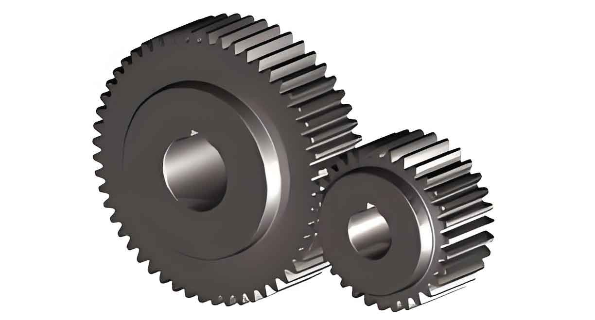
The potential energy method, first introduced by Yang et al., relies on calculating the potential energy stored in meshing spur gears to determine stiffness. The total potential energy is composed of several components: Hertzian contact energy, bending energy, shear energy, axial compression energy, and gear body energy. Each corresponds to a specific stiffness: Hertzian contact stiffness \(k_h\), bending stiffness \(k_b\), shear stiffness \(k_s\), axial compression stiffness \(k_a\), and gear body stiffness \(k_f\). For a pair of meshing spur gears, the total potential energy \(U\) is given by:
$$U = \frac{F^2}{2k} = U_h + U_{b1} + U_{s1} + U_{a1} + U_{f1} + U_{b2} + U_{s2} + U_{a2} + U_{f2}$$
where \(F\) is the meshing force, and subscripts 1 and 2 denote the driving and driven spur gears, respectively. The individual energy components are expressed as:
$$U_h = \frac{F^2}{2k_h}, \quad U_b = \frac{F^2}{2k_b}, \quad U_s = \frac{F^2}{2k_s}, \quad U_a = \frac{F^2}{2k_a}, \quad U_f = \frac{F^2}{2k_f}$$
The Hertzian contact stiffness for spur gears is calculated using:
$$k_h = \frac{\pi E L}{4(1 – \nu^2)}$$
where \(E\) is the elastic modulus, \(L\) is the tooth width, and \(\nu\) is Poisson’s ratio. The gear body stiffness, accounting for the ring structure, is derived from Sainsot et al. as:
$$\frac{1}{k_f} = \frac{\cos^2 \beta}{E L} \left[ L^* \left( \frac{u_f}{S_f} \right)^2 + M^* \left( \frac{u_f}{S_f} \right) + P^* (1 + Q^* \tan^2 \beta) \right]$$
where \(\beta\) is the helix angle (zero for spur gears), and \(L^*, M^*, P^*, Q^*\) are coefficients based on gear geometry. For spur gears with \(\beta = 0\), this simplifies to:
$$\frac{1}{k_f} = \frac{1}{E L} \left[ L^* \left( \frac{u_f}{S_f} \right)^2 + M^* \left( \frac{u_f}{S_f} \right) + P^* \right]$$
In the meshing process of spur gears, different zones exist: single-tooth contact and double-tooth contact. The overall meshing stiffness \(k\) for a spur gear pair is computed as follows. For the single-tooth contact zone:
$$\frac{1}{k} = \frac{1}{k_h} + \sum_{i=1,2} \left( \frac{1}{k_{b,i}} + \frac{1}{k_{s,i}} + \frac{1}{k_{a,i}} + \frac{1}{k_{f,i}} \right)$$
For the double-tooth contact zone, where two pairs of teeth are engaged:
$$\frac{1}{k} = \sum_{j=1}^{2} \left( \frac{1}{k_h} + \sum_{i=1,2} \left( \frac{1}{k_{b,i,j}} + \frac{1}{k_{s,i,j}} + \frac{1}{k_{a,i,j}} + \frac{1}{k_{f,i,j}} \right) \right)$$
These formulas form the basis for TVMS calculation, but they require accurate models of tooth deformation. Previous studies often simplified the tooth profile, leading to errors, especially for spur gears with higher tooth counts. Our improvement focuses on the full tooth profile of spur gears, dividing it into the involute part and the transition curve part. The transition curve, generated by the rack-type cutter with a rounded tip, is described by a parametric equation. For spur gears, the coordinates \((x_1, y_1)\) of the transition curve are given by:
$$x_1 = r \cos \phi – (a / \sin \gamma + \rho) \sin(\gamma – \phi)$$
$$y_1 = r \sin \phi – (a / \sin \gamma + \rho) \cos(\gamma – \phi)$$
where \(r\) is the pitch radius, \(\phi = (a \tan \gamma + b)/r\), \(a = h_a^* m + c^* m – \rho\), \(b = \pi m/4 + h_a^* m \tan \alpha_0 + \rho \cos \alpha_0\), \(\rho = c^* m / (1 – \sin \alpha_0)\), \(m\) is the module, \(h_a^*\) is the addendum coefficient, \(c^*\) is the clearance coefficient, \(\alpha_0\) is the pressure angle, and \(\gamma\) is a parameter ranging from \(\alpha_0\) to \(\pi/2\). This parametric representation ensures accuracy for all spur gears, regardless of tooth number.
The key innovation in our method for spur gears lies in addressing the relationship between the radii of the involute start point \(r_G\), base circle \(r_b\), and root circle \(r_f\). These radii are defined as:
$$r_b = \frac{m N \cos \alpha_0}{2}, \quad r_f = \frac{m N}{2} – (h_a^* + c^*) m, \quad r_G = \sqrt{r^2 + (a / \sin \alpha_0 + \rho)^2 – 2r(a + \rho \sin \alpha_0)}$$
where \(N\) is the number of teeth. For standard spur gears, when \(N = 17.10\), \(r_G = r_b\), and when \(N = 41.25\), \(r_f = r_b\). In traditional models, the involute profile is assumed to start from the base circle, but for spur gears with \(N > 41\), the base circle lies inside the root circle, causing a discrepancy between \(r_G\) and \(r_b\). This leads to errors in stiffness calculation if not corrected. We categorize spur gears based on tooth count:
- Case 1: \(17 < N \leq 41\) – The base circle is above the root circle, and the involute starts near the base circle.
- Case 2: \(N > 41\) – The base circle is below the root circle, and the involute start point \(G\) deviates from the base circle point \(G_b\).
For spur gears in Case 1, the traditional integral limits for the involute part are valid. The bending, shear, and axial compression stiffness for the involute profile are calculated as:
$$\frac{1}{k_b} = \int_{-\alpha_1}^{\alpha_2} \frac{3(\alpha_2 – \alpha) \cos \alpha}{2EL [\sin \alpha + (\alpha_2 – \alpha) \cos \alpha]^3} \left\{ 1 + \cos \alpha_1 [(\alpha_2 – \alpha_1) \sin \alpha – \cos \alpha] \right\}^2 d\alpha$$
$$\frac{1}{k_s} = \int_{-\alpha_1}^{\alpha_2} \frac{1.2(1 + \nu)(\alpha_2 – \alpha) \cos \alpha \cos^2 \alpha_1}{EL [\sin \alpha + (\alpha_2 – \alpha) \cos \alpha]} d\alpha$$
$$\frac{1}{k_a} = \int_{-\alpha_1}^{\alpha_2} \frac{(\alpha_2 – \alpha) \cos \alpha \sin^2 \alpha_1}{2EL [\sin \alpha + (\alpha_2 – \alpha) \cos \alpha]} d\alpha$$
where \(\alpha_1\) is the pressure angle at the meshing point, \(\alpha_2 = \pi/(2N) + \text{inv} \alpha_0\) is the half-base tooth angle, and \(\text{inv} \alpha_0 = \tan \alpha_0 – \alpha_0\). For spur gears in Case 2, we modify the integral upper limit from \(\alpha_2\) to \(\alpha_G\), where \(\alpha_G\) is the pressure angle at the involute start point \(G\), given by:
$$\alpha_G = \arccos \left( \frac{r_b}{r_G} \right) – \left( \frac{\pi}{2N} + \text{inv} \alpha_0 – \text{inv} \alpha_G \right)$$
This adjustment accounts for the actual involute profile in spur gears. The corrected stiffness formulas become:
$$\frac{1}{k_b} = \int_{-\alpha_1}^{\alpha_G} \frac{3(\alpha_2 – \alpha) \cos \alpha}{2EL [\sin \alpha + (\alpha_2 – \alpha) \cos \alpha]^3} \left\{ 1 + \cos \alpha_1 [(\alpha_2 – \alpha_1) \sin \alpha – \cos \alpha] \right\}^2 d\alpha$$
$$\frac{1}{k_s} = \int_{-\alpha_1}^{\alpha_G} \frac{1.2(1 + \nu)(\alpha_2 – \alpha) \cos \alpha \cos^2 \alpha_1}{EL [\sin \alpha + (\alpha_2 – \alpha) \cos \alpha]} d\alpha$$
$$\frac{1}{k_a} = \int_{-\alpha_1}^{\alpha_G} \frac{(\alpha_2 – \alpha) \cos \alpha \sin^2 \alpha_1}{2EL [\sin \alpha + (\alpha_2 – \alpha) \cos \alpha]} d\alpha$$
For the transition curve part of spur gears, the stiffness components are derived using the parametric equations. The bending, shear, and axial compression stiffness are expressed as integrals over the parameter \(\gamma\):
$$\frac{1}{k_b} = \int_{\alpha_0}^{\pi/2} \frac{[\cos \alpha_1 (l – y_1) – h \sin \alpha_1]^2}{E I_{y_1}} \frac{dy_1}{d\gamma} d\gamma$$
$$\frac{1}{k_s} = \int_{\alpha_0}^{\pi/2} \frac{1.2 \cos^2 \alpha_1}{G A_{y_1}} \frac{dy_1}{d\gamma} d\gamma$$
$$\frac{1}{k_a} = \int_{\alpha_0}^{\pi/2} \frac{\sin^2 \alpha_1}{E A_{y_1}} \frac{dy_1}{d\gamma} d\gamma$$
where \(I_{y_1} = 2x_1^3 L/3\) and \(A_{y_1} = 2x_1 L\) are the moment of inertia and cross-sectional area at point \((x_1, y_1)\), \(G = E/[2(1+\nu)]\) is the shear modulus, \(l = r_b \cos \alpha_1 + r_b (\alpha_1 + \alpha_2) \sin \alpha_1\), and \(h = r_b (\alpha_1 + \alpha_2) \cos \alpha_1 – r_b \sin \alpha_1\). The derivative \(dy_1/d\gamma\) is computed from the parametric equations.
The total stiffness for a spur gear tooth is the sum of the transition curve and involute parts. For spur gears with \(17 < N \leq 41\):
$$\frac{1}{k_b} = \int_{\alpha_0}^{\pi/2} \frac{[\cos \alpha_1 (l – y_1) – h \sin \alpha_1]^2}{E I_{y_1}} \frac{dy_1}{d\gamma} d\gamma + \int_{-\alpha_1}^{\alpha_2} \frac{3(\alpha_2 – \alpha) \cos \alpha}{2EL [\sin \alpha + (\alpha_2 – \alpha) \cos \alpha]^3} \left\{ 1 + \cos \alpha_1 [(\alpha_2 – \alpha_1) \sin \alpha – \cos \alpha] \right\}^2 d\alpha$$
For spur gears with \(N > 41\):
$$\frac{1}{k_b} = \int_{\alpha_0}^{\pi/2} \frac{[\cos \alpha_1 (l – y_1) – h \sin \alpha_1]^2}{E I_{y_1}} \frac{dy_1}{d\gamma} d\gamma + \int_{-\alpha_1}^{\alpha_G} \frac{3(\alpha_2 – \alpha) \cos \alpha}{2EL [\sin \alpha + (\alpha_2 – \alpha) \cos \alpha]^3} \left\{ 1 + \cos \alpha_1 [(\alpha_2 – \alpha_1) \sin \alpha – \cos \alpha] \right\}^2 d\alpha$$
Similar expressions apply to shear and axial compression stiffness. These formulas provide a comprehensive model for TVMS calculation in spur gears, ensuring accuracy across different tooth counts.
To validate our improved method for spur gears, we conduct case studies comparing it with traditional approaches and finite element analysis. We consider four spur gear pairs with varying tooth numbers: Pair A with \(N_1 = N_2 = 22\), Pair B with \(N_1 = N_2 = 42\), Pair C with \(N_1 = N_2 = 62\), and Pair D with \(N_1 = 19\) and \(N_2 = 48\). The gear parameters are: module \(m = 3 \, \text{mm}\), pressure angle \(\alpha_0 = 20^\circ\), addendum coefficient \(h_a^* = 1\), clearance coefficient \(c^* = 0.25\), tooth width \(L = 20 \, \text{mm}\), elastic modulus \(E = 2.06 \times 10^{11} \, \text{Pa}\), and Poisson’s ratio \(\nu = 0.3\). We define Method A as the traditional potential energy method with transition curve consideration but without integral limit modification, Method B as our improved method, and FEM as the finite element method reference.
The TVMS results for each spur gear pair are summarized in the tables below. Table 1 shows the maximum single-tooth meshing stiffness and average TVMS values, along with relative errors compared to Method A.
| Gear Pair | Method | Max Single-Tooth Stiffness (10^8 N/m) | Average TVMS (10^8 N/m) | Relative Error vs. Method A (%) |
|---|---|---|---|---|
| Pair A: N1=N2=22 | Method A | 2.62 | 3.56 | 0 |
| Method B | 2.53 | 3.55 | 0.28 | |
| FEM | 2.51 | 3.45 | 3.09 | |
| Pair B: N1=N2=42 | Method A | 2.74 | 3.80 | 0 |
| Method B | 2.64 | 3.76 | 1.05 | |
| FEM | 2.61 | 3.65 | 3.95 | |
| Pair C: N1=N2=62 | Method A | 2.73 | 3.81 | 0 |
| Method B | 2.62 | 3.75 | 1.57 | |
| FEM | 2.60 | 3.66 | 3.94 | |
| Pair D: N1=19, N2=48 | Method A | 2.65 | 3.62 | 0 |
| Method B | 2.52 | 3.56 | 1.66 | |
| FEM | 2.51 | 3.50 | 3.31 |
From Table 1, we observe that for spur gears with lower tooth counts (e.g., Pair A), the error between Methods A and B is minimal (0.28% for average TVMS), as the involute start point and base circle are nearly coincident. However, for spur gears with higher tooth counts (Pairs B and C), the error increases, reaching 1.57% for Pair C. This confirms that the discrepancy between \(r_G\) and \(r_b\) becomes significant as tooth number rises, leading to larger calculation errors if not corrected. For Pair D, where the spur gears have differing tooth numbers, the error is 1.66%, highlighting the importance of using separate models for each gear in a pair. In all cases, Method B shows closer agreement with FEM results than Method A, validating our improved approach for spur gears.
To further analyze the impact of tooth number on TVMS in spur gears, we compute the stiffness over a full meshing cycle. The TVMS curves for each pair are derived using the formulas above. For spur gears, the meshing stiffness varies periodically due to changing contact conditions. The stiffness values at key points, such as the pitch point and the start/end of contact, are critical for dynamic analysis. We present additional data in Table 2, focusing on the stiffness contributions from different components for a sample spur gear with \(N=42\).
| Component | Stiffness Value (10^8 N/m) | Percentage of Total (%) |
|---|---|---|
| Hertzian Contact Stiffness \(k_h\) | 15.32 | ~40 |
| Bending Stiffness \(k_b\) | 8.45 | ~22 |
| Shear Stiffness \(k_s\) | 6.78 | ~18 |
| Axial Compression Stiffness \(k_a\) | 4.21 | ~11 |
| Gear Body Stiffness \(k_f\) | 3.89 | ~10 |
| Total Single-Tooth Stiffness | 2.64 | 100 |
This breakdown illustrates the relative importance of each stiffness component in spur gears, with Hertzian contact and bending stiffness being dominant. Our improved method refines the bending and shear calculations by accurately modeling the tooth profile.
The mathematical derivation for spur gears can be extended to include effects like cracks or wear, but here we focus on healthy gears. The potential energy stored in a spur gear tooth under load \(F\) is also influenced by the contact ratio. For spur gears, the contact ratio \(CR\) is given by:
$$CR = \frac{\sqrt{r_{a1}^2 – r_{b1}^2} + \sqrt{r_{a2}^2 – r_{b2}^2} – a \sin \alpha_0}{\pi m \cos \alpha_0}$$
where \(r_{a1}\) and \(r_{a2}\) are the addendum radii of the spur gears, and \(a\) is the center distance. A higher contact ratio in spur gears often leads to smoother TVMS transitions. Our method accounts for this through the double-tooth contact formulas.
In terms of computational efficiency, the improved potential energy method for spur gears offers advantages over FEM. The analytical formulas reduce calculation time while maintaining accuracy. For instance, the stiffness integrals can be solved numerically using techniques like Gaussian quadrature. We recommend the following steps for implementing our method for spur gears:
- Determine the tooth number \(N\) for each spur gear in the pair.
- Calculate \(r_b\), \(r_f\), and \(r_G\) using the formulas above.
- Classify the gear into Case 1 or Case 2 based on \(N\).
- Compute the transition curve stiffness using the parametric integrals.
- Compute the involute stiffness with the appropriate integral limits (\(\alpha_2\) or \(\alpha_G\)).
- Sum the stiffness components and incorporate Hertzian and gear body stiffness.
- Repeat for each meshing position to obtain the TVMS curve.
To further justify our improvements for spur gears, we analyze the error sources. The primary error in traditional methods stems from assuming the involute starts at the base circle. For spur gears with \(N > 41\), this assumption introduces an overestimation of the involute profile length, leading to higher calculated stiffness. Our correction reduces this by limiting the integral to \(\alpha_G\). The error magnitude \(\Delta k\) can be estimated as:
$$\Delta k \approx \int_{\alpha_G}^{\alpha_2} f(\alpha) d\alpha$$
where \(f(\alpha)\) represents the integrand in the stiffness formulas. As \(N\) increases, \(\alpha_2 – \alpha_G\) grows, so \(\Delta k\) increases, consistent with our results. For spur gears with \(N \leq 41\), \(\alpha_G \approx \alpha_2\), so \(\Delta k\) is negligible.
Additionally, the transition curve modeling in spur gears is crucial for accuracy. Simplifying the transition curve as a straight line, as in some studies, can cause errors of up to 5% in TVMS. Our parametric equation captures the exact geometry, especially for spur gears manufactured via rack-type cutters. The impact of cutter parameters like \(\rho\) on TVMS is significant; for example, a larger \(\rho\) increases the transition curve length, slightly reducing stiffness. We explore this through parametric studies in Table 3 for a spur gear with \(N=50\).
| Cutter Radius \(\rho\) (mm) | Average TVMS (10^8 N/m) | Change vs. Baseline (%) |
|---|---|---|
| 0.5 (Baseline) | 3.70 | 0 |
| 0.75 | 3.67 | -0.81 |
| 1.00 | 3.64 | -1.62 |
| 1.25 | 3.61 | -2.43 |
This table shows that as \(\rho\) increases, the TVMS decreases slightly due to a more gradual transition curve, which affects the bending and shear stiffness in spur gears. Our method incorporates \(\rho\) explicitly, allowing for precise analysis.
In conclusion, our improved potential energy method for spur gears enhances the calculation of time-varying meshing stiffness by considering the full tooth profile and adjusting integral limits based on tooth number. We divide the spur gear tooth into involute and transition curve parts, using parametric equations for accuracy. For spur gears with tooth numbers greater than 41, we modify the integral upper limit to account for the deviation between the involute start point and base circle. Case studies demonstrate that errors from traditional methods increase with tooth number, and for spur gear pairs with differing tooth counts, separate models are necessary to avoid significant errors. The results align well with finite element analysis, validating our approach. This method provides a reliable, efficient tool for dynamic analysis of spur gears in applications like automotive transmissions and industrial machinery. Future work could extend this to helical gears or include fault conditions, but the core principles for spur gears remain foundational.
The formulas and tables presented here offer a comprehensive framework for engineers and researchers working with spur gears. By implementing these improvements, the prediction of vibration and noise in spur gear systems can be enhanced, leading to better design and maintenance practices. The emphasis on spur gears throughout this study underscores their importance in mechanical engineering, and our methodological refinements contribute to the ongoing advancement of gear dynamics.