
The precision of the helix angle in helical gears is a critical determinant for the smoothness, noise level, and service life of mechanical transmission systems. Traditional methods for analyzing the helix angle of helical gears, such as geometric projection-based measurements and contact-probe-based detection, possess inherent limitations. These methods often fail to capture the minute variations along the tooth flank and adequately account for the dynamic coupling effects among various geometric parameters. This inadequacy leads to inaccuracies in calculating the tangent relationship between the helix angle at the pitch circle and that at the tip circle, consequently resulting in significant uncertainty and error in the measurement of helix angle deviation. Therefore, developing a high-precision detection algorithm capable of overcoming these limitations is of substantial practical importance for ensuring the machining quality of machine tool helical gears.
The tooth line of a helical gear can be conceptualized as a set of helices wound around a cylindrical surface. To establish a mathematical foundation, the parametric equations for a helix are derived within a three-dimensional Cartesian coordinate system.
$$ \begin{cases}
x = r \times \cos\left( \theta_0 + \theta + \frac{2\pi n}{c} \right) \\
y = r \times \sin\left( \theta_0 + \theta + \frac{2\pi n}{c} \right) \\
z = \pm b \times \theta = \pm r \times \theta \times \cot \beta = \pm \frac{r \times \theta}{\tan \beta}
\end{cases} $$
where:
- $r$ is the radius of the cylindrical surface (corresponding to the pitch or tip radius of the helical gear),
- $c$ is the number of teeth,
- $b$ is the axial displacement per radian of rotation, related to the lead,
- $\theta$ is the angular parameter (in radians), ranging within $(-b/r, 0)$ or equivalent,
- $n$ is an integer representing the specific helix (tooth),
- $\pi$ is the mathematical constant,
- $\beta$ is the helix angle at the reference cylinder (pitch cylinder),
- $\theta_0$ is the initial phase angle.
In the transverse plane coordinate system, the arc of rotation for each helix on a helical gear is $2\pi n / c$. The sign of $r$ and $b$ determines the hand of the helix (left-handed or right-handed).
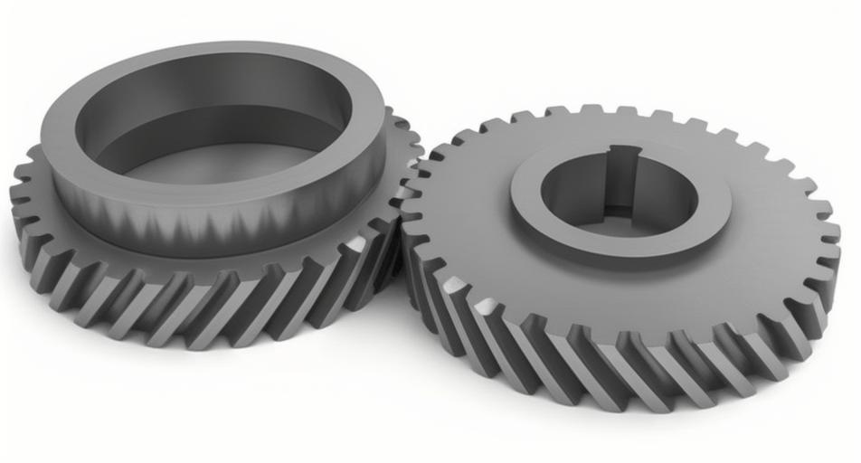
Analysis of the projection reveals that the helix is not a straight line but approximates one. From the parametric equations, the functional relationship between $x$ and $z$ can be expressed as:
$$ x = r \times \cos\left( \theta_0 + \frac{z \times \tan \beta}{r} + \frac{2\pi n}{c} \right) $$
Assuming the gear axis intersects the upper end face at point $(x_0, z_0)$, a more comprehensive relationship incorporating all coordinates is:
$$ \begin{cases}
z = h(y) \\
x = r \times \cos\left( \frac{\pi}{2} – \arctan\left(\frac{x – x_0}{z – z_0}\right) + \frac{2\pi n}{c} + \theta_0 \right)
\end{cases} $$
Typically, the tip diameter $d_y$ of a helical gear is related to the pitch diameter $d$ and the module $m$. The helix angles at the pitch circle $\beta$ and the tip circle $\beta_y$ are defined by their tangents, which are functions of the axial lead $P_z$ and the respective diameters:
$$ \tan \beta = \frac{P_z}{\pi d} $$
$$ \tan \beta_y = \frac{P_z}{\pi d_y} $$
Where $P_z$ is the lead of the helical tooth surface. For standard helical gears, $d = m \times c$ and $d_y = d + 2m$. The derivation of these tangent values from the fundamental parametric equations addresses the core computational challenge neglected by traditional methods, providing a precise mathematical model for the helix angle relationship.
While the theoretical tangent values provide the foundation, determining the actual helix angle requires accounting for real-world manufacturing imperfections. Theoretical models assume ideal conditions, but actual helical gear production is influenced by machine tool accuracy, tool wear, and other process variables. Therefore, a direct measurement technique is essential. This algorithm employs a laser interferometer to measure key parameters, combines them with the derived tangent relationships to compute the actual helix angle, and finally compares it with the standard value to ascertain the deviation.
The principle relies on the optical feedback phenomenon in laser interferometry. The laser interferometer emits a beam with two polarization frequencies, $f_1$ and $f_2$. A reference signal at frequency $f_1 – f_2$ is generated. The beam is split by an interferometric optic, directing $f_1$ and $f_2$ to a fixed reference mirror and a moving mirror attached to the measurement axis (simulating gear rotation or probe movement), respectively. The reflected beams recombine at the beam splitter and return to the interferometer’s detector. After photodetection and processing, a measurement signal with frequency $f_1 – f_2 \pm \Delta f$ is produced, where $\Delta f$ is the Doppler shift induced by the mirror’s velocity $v$. The frequency of the reflected beam after interference is given by:
$$ f_1 – f_2 \pm \Delta f \approx (f_1 – f_2) \left(1 – \frac{2v}{a}\right) $$
where $a$ is the speed of light. The displacement $l$ is obtained by integrating the velocity signal derived from $\Delta f$. The laser interference phase equation, considering optical feedback from the gear surface, is modeled as:
$$ s_F(t) = s_0(t) + \lambda \left[ \sin(\arctan(s_0(t))) + C \times s_0(t) \right] $$
where:
- $\lambda$ is the laser wavelength,
- $s_0(t)$ is the phase of the laser external cavity without optical feedback,
- $s_F(t)$ is the phase with optical feedback,
- $C$ is the optical feedback coefficient,
- $\alpha$ is the linewidth enhancement factor.
With a sampling frequency set at 50 kHz, the phase signal $s_0(t)$ is used to measure and acquire signals related to the helical gear‘s module, number of teeth, rotation angle, and tooth width. These signals are processed in a computational environment like MATLAB.
Parameter Measurement via Laser Interferometry and Image Processing:
- Module ($m$): The gear tooth profiles are extracted. Connecting points on each tooth forms a convex polygon. Using the laser interferometer’s positioning and imaging capabilities, coupled with a reflective target, the optical feedback coefficient $C$ is determined. A circle with radius $R_k$ is fitted to the polygon vertices using the least squares method. The center is $(x’, y’)$. The radius $R_j$ of the maximum inscribed circle within this polygon is found. The module is then calculated by referencing a standard module table value $M$ (e.g., 2.25):
$$ m = \frac{R_k – R_j}{M} $$
- Number of Teeth ($c$): A circle centered at $(x’_1, y’_1)$ with radius $(R_k + R_j)/2$ is projected onto the gear image via the laser interferometer system. After processing the phase signal $s_0(t)$ and applying binarization, a clear tooth form image is obtained, from which the actual number of teeth $c$ is counted directly.
- Rotation Angle ($\gamma$): The gear is rotated about the axis defined by the center of the upper end face until the calculated tangents of the helix angles at the measured pitch and tip circles match the values derived from the parametric equations ($\tan \beta$ and $\tan \beta_y$). The minimum angle of this rotation is $\gamma$. It can be calculated using the law of cosines based on coordinates of the center on the upper face, the lower face, and the gear center:
$$ \gamma = \arccos\left( \frac{s_1^2 + s_2^2 – s_3^2}{2 s_1 s_2} \right) $$
where $s_1$ and $s_2$ are distances from the upper and lower face center coordinates to the gear center coordinate, respectively, and $s_3$ is the distance between the upper and lower face center coordinates.
- Face Width ($h$): The face width is measured directly using a precision caliper or can be derived from axial scan data from the interferometer.
Helix Angle Calculation and Deviation Determination:
Using the measured parameters, the actual helix angle $\beta_{\text{actual}}$ of the machine tool helical gear is calculated with the following formula, which stems from the geometric relationship defined by the helix lead:
$$ \tan \beta_{\text{actual}} = \frac{\pi \cdot c \cdot m}{h} \cdot \frac{\gamma}{360} $$
Note: $\gamma$ here is in degrees for this formula, ensuring consistency with the $360$ in the denominator. Finally, the helix angle deviation $\Delta \beta$ is obtained by comparing the calculated actual value with the standard specified value $\beta_{\text{std}}$:
$$ \Delta \beta = \beta_{\text{actual}} – \beta_{\text{std}} $$
Experimental Validation and Performance Comparison:
To validate the practical efficacy of the proposed Laser Interference Detection Algorithm for the precise detection of helix angle deviation in machine tool helical gears, comparative experiments were conducted against the traditional “Roll-Grinding” process calculation method and a parametric visual inspection method.
Experimental Setup and Parameters:
The test specimen was a helical gear with the following specifications: Tip diameter = 32.00 mm, Pitch diameter = 35.66 mm, Number of teeth = 25, Module = 1.25 mm, Material = 45 Steel. Key measurement equipment included:
- Laser Interferometer (Renishaw XL-80, accuracy ±0.1 µm) for the proposed method.
- High-precision rotary table (accuracy ±1 arcsecond).
- Industrial Camera (5 Megapixel resolution) for the visual inspection method.
Experimental Procedure & Data Analysis:
The proposed method was first validated for its core step of deriving accurate tangent values. Over 10 experimental runs, the helical gear was deliberately placed at slightly different angular orientations. For each run, the actual helix angle was calculated using the derived formulas based on interferometric measurements. The deviation from the standard helix angle ($\beta_{\text{std}} = 19.32^\circ$) was recorded, as shown in Table 1.
| Experiment No. | Actual Helix Angle $\beta_{\text{actual}}$ (°) | Standard Helix Angle $\beta_{\text{std}}$ (°) | Deviation $\Delta \beta$ (°) |
|---|---|---|---|
| 1 | 19.41 | 19.32 | 0.09 |
| 2 | 19.40 | 19.32 | 0.08 |
| 3 | 19.42 | 19.32 | 0.10 |
| 4 | 19.43 | 19.32 | 0.11 |
| 5 | 19.42 | 19.32 | 0.10 |
| 6 | 19.44 | 19.32 | 0.12 |
| 7 | 19.45 | 19.32 | 0.13 |
| 8 | 19.40 | 19.32 | 0.08 |
| 9 | 19.41 | 19.32 | 0.09 |
| 10 | 19.42 | 19.32 | 0.10 |
The results demonstrate small and stable deviation values, confirming that the deep analytical derivation of the helix parametric equations provides a reliable data foundation for precise helix angle calculation in helical gears.
Subsequently, to evaluate detection performance, all three methods were used to detect the helix angle deviation over 60 experimental runs. The relative error $E_r$ for each method was calculated against known, introduced deviations using the formula:
$$ E_r = \frac{|l – l_0|}{l_0} \times 100\% $$
where $l_0$ is the actual (introduced) deviation value and $l$ is the value detected by the algorithm. The comparative results consistently showed that the proposed laser interference method achieved the smallest $E_r$ values, followed by the parametric visual method, with the “Roll-Grinding” method exhibiting the largest errors. This confirms the superior accuracy of the proposed algorithm for helical gear inspection.
A robustness test involved 50 detection cycles with specific, artificially introduced helix angle deviations during experiments 10, 15, 20, 25, 35, 40, and 45. The proposed method accurately identified and quantified these introduced deviations with high stability and precision throughout the test sequence. In contrast, the “Roll-Grinding” and visual inspection methods showed significant detection inaccuracies and instability when faced with these deliberate changes, indicating poorer adaptability to complex, variable conditions common in real-world helical gear manufacturing and inspection environments.
Finally, to simulate a complex operational environment with uncertainties like thermal effects and vibrations, each method performed 10 helix angle deviation detection tests. The fluctuation range (difference between maximum and minimum detected deviation) was recorded for each algorithm, as summarized in Table 2.
| Detection Method | Fluctuation Range of $\Delta \beta$ (°) |
|---|---|
| Proposed Laser Interference Method | ±1.5 |
| “Roll-Grinding” Process Calculation Method | ±3.5 |
| Parametric Visual Inspection Method | ±5.5 |
The proposed algorithm demonstrated the smallest fluctuation range (±1.5°), indicating significantly higher stability and reliability in complex, noisy environments compared to the traditional “Roll-Grinding” method (±3.5°) and the visual inspection method (±5.5°).
Conclusion:
This research addressed the critical challenge of precise helix angle deviation detection in machine tool helical gears. The proposed Laser Interference Detection Algorithm fundamentally improves upon traditional methods by:
- Establishing a precise mathematical model through deep derivation of helix parametric equations, yielding accurate tangent relationships for the pitch and tip circle helix angles.
- Integrating high-precision laser interferometric measurements of key gear parameters (module, tooth count, rotation angle) with the derived model to calculate the actual helix angle, achieving a maximum relative error not exceeding 0.13° in controlled tests.
- Demonstrating exceptional stability with a helix angle deviation fluctuation range constrained within ±1.5° under simulated complex conditions, substantially outperforming the “Roll-Grinding” (±3.5°) and visual inspection (±5.5°) methods.
The algorithm provides a robust, high-precision, and stable solution for inspecting helix angle deviation in helical gears, thereby offering a reliable means to safeguard and enhance the machining accuracy of critical gear components in advanced manufacturing systems.