
I study face gears because they combine high contact ratio, favorable torque splitting, and the absence of axial force on the pinion. These features make face gears attractive for compact, high-power transmissions. However, the real meshing state of face gears is strongly affected by manufacturing errors, assembly errors, and elastic deformation. Under such conditions, edge contact can occur at the tooth tip or at the inner radius, producing severe stress concentration and reducing durability. At the same time, the generated tooth surface of face gears has a continuously varying profile and complex topology. When modification is introduced, the geometric complexity increases further. Conventional analytical loaded contact analysis becomes difficult to apply directly, while general finite element simulation remains accurate but computationally expensive. I therefore develop a localized line contact modification method for face gears and an efficient numerical loaded contact model based on the influence coefficient method.
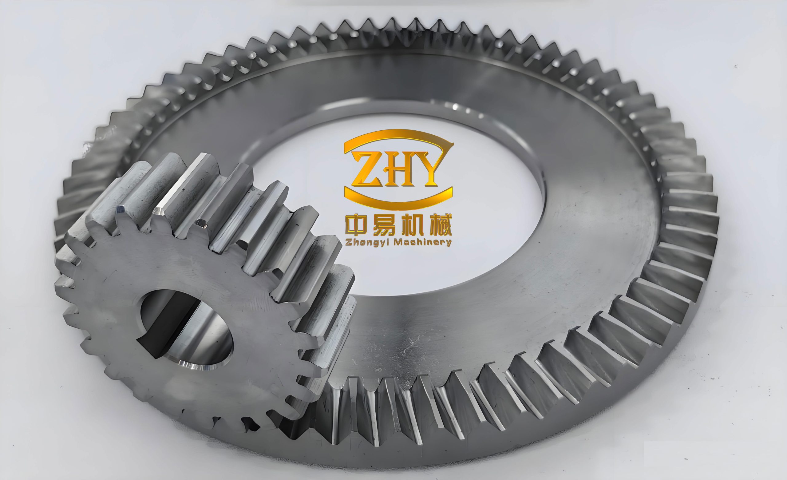
My objective is to improve the load capacity of face gears, avoid edge contact, and preserve a high level of computational efficiency for iterative design. I discretize the standard face gear tooth surface using contact lines. I then superimpose modification amounts on discrete nodes along the contact line and along a predetermined contact path. In this way, I construct a geometric model of face gears with localized line contact characteristics. After that, I build a mesh model from the modified geometry. I establish a tooth-surface force-displacement response matrix using the influence coefficient method. I combine deformation compatibility equations and moment equilibrium conditions to compute the contact stress and load distribution of face gears. Finally, I verify the modification method and the numerical model. The results show that the predetermined contact path agrees with the simulated contact path, the contact stress computed by my numerical method agrees well with Abaqus results, and the computational efficiency is significantly improved. Compared with point contact, localized line contact reduces the maximum contact stress and avoids edge contact in face gears.
Contact strategies for face gears. The contact form of face gears directly controls load capacity and error sensitivity. A full line contact preserves a continuous contact line across the tooth width and therefore has high theoretical load capacity, but it is extremely sensitive to assembly errors. A point contact reduces sensitivity and confines the contact area, but it sacrifices load-carrying area and can still produce tip edge contact. A localized line contact is a compromise: it creates a controlled contact line on a predetermined path, retains a large contact area, and keeps the contact zone away from tooth boundaries. I summarize the three strategies in Table 1.
| Contact strategy | Contact area | Load capacity | Error sensitivity | Edge contact risk |
|---|---|---|---|---|
| Full line contact | Continuous across full tooth width | Highest theoretical value | Highest | High at tip and inner radius |
| Point contact | Small ellipse or point-like zone | Lower due to small area | Lowest | Moderate at tooth tip |
| Localized line contact | Controlled line segment | High and stable | Moderate | Low within a certain error range |
Geometric generation of standard face gears. I generate the standard face gear tooth surface by simulating the meshing motion between a shaper cutter and the face gear. The shaper cutter is a cylindrical gear whose geometric parameters match the pinion. The cutter tooth surface can be written as a function of two surface parameters. I define the cutter surface as
$$
\mathbf r_b(u_b,\theta_b)=
\begin{bmatrix}
r_{bs}\left[\sin(\theta_{bs}+\theta_b)-\theta_b\cos(\theta_{bs}+\theta_b)\right]\\
-r_{bs}\left[\cos(\theta_{bs}+\theta_b)+\theta_b\sin(\theta_{bs}+\theta_b)\right]\\
u_b\\
1
\end{bmatrix}
$$
where \(u_b\) is the coordinate along the cutter tooth width, \(\theta_b\) is the involute angle parameter, \(r_{bs}\) is the base radius of the shaper cutter, and \(\theta_{bs}\) is the half angle of the cutter tooth space. The transformation from the cutter coordinate system to the face gear coordinate system is
$$
\mathbf r_2=\mathbf M_{2b}(\phi_b)\mathbf r_b
$$
where \(\phi_b\) is the rotation angle of the shaper cutter relative to the face gear. The matrix \(\mathbf M_{2b}\) contains the relative position and orientation of the two coordinate systems. A general form of this matrix is
$$
\mathbf M_{2b}(\phi_b)=
\begin{bmatrix}
c\phi_b c\phi_m-s\phi_b s\phi_m c\gamma_m & -c\phi_b s\phi_m-s\phi_b c\phi_m c\gamma_m & s\phi_b s\gamma_m & 0\\
s\phi_b c\phi_m+c\phi_b s\phi_m c\gamma_m & -s\phi_b s\phi_m+c\phi_b c\phi_m c\gamma_m & -c\phi_b s\gamma_m & 0\\
s\phi_m s\gamma_m & c\phi_m s\gamma_m & c\gamma_m & 0\\
0 & 0 & 0 & 1
\end{bmatrix}
$$
In the matrix, \(c\) and \(s\) denote cosine and sine, \(\phi_m\) is the mounting angle, and \(\gamma_m\) is the shaft angle. The meshing equation of the generation process is obtained from the condition that the relative velocity is perpendicular to the common normal:
$$
f(u_b,\theta_b,\phi_b)=\mathbf n_b\cdot \mathbf v_b^{(2m)}=0
$$
For the involute shaper cutter and the face gear generation motion, this equation can be expanded as
$$
f(u_b,\theta_b,\phi_b)=
(1-\cos\gamma_m)u_b+
\sin\gamma_m\left[r_{bs}\cos(\theta_{bs}+\theta_b)-\theta_b\sin(\theta_{bs}+\theta_b)\right]
-\cos\gamma_m\left[r_{bs}\sin(\theta_{bs}+\theta_b)+\theta_b\cos(\theta_{bs}+\theta_b)\right]=0
$$
By combining the meshing equation with the coordinate transformation, I obtain the standard face gear tooth surface:
$$
\mathbf r_2(u_b,\theta_b)=\mathbf M_{2b}(\phi_b(u_b,\theta_b))\mathbf r_b(u_b,\theta_b),
\quad
f(u_b,\theta_b,\phi_b(u_b,\theta_b))=0
$$
The standard face gear surface is therefore a generated envelope surface. Its local geometry changes continuously from the inner radius to the outer radius and from the root to the tip. This variation is one of the main reasons why a general analytical contact model for face gears is difficult to construct. I use a digital discretization strategy instead. I divide the tooth surface along contact lines and store the position and normal vector at every discrete node. The discrete model is then used both for modification and for the numerical loaded contact analysis.
Localized line contact modification. I introduce modification on the contact lines that appear during the generation of face gears. I first define a predetermined contact path on the tooth surface. I select two end points \(\mathbf m_1\) and \(\mathbf m_2\). Their midpoint is
$$
\mathbf M=\frac{\mathbf m_1+\mathbf m_2}{2}
$$
The direction of the contact path is
$$
\hat{\mathbf u}=\frac{\mathbf m_2-\mathbf m_1}{\|\mathbf m_2-\mathbf m_1\|}
$$
I choose a direction \(\hat{\mathbf a}\) perpendicular to \(\hat{\mathbf u}\). The contact path is represented by a parabolic curve:
$$
\mathbf c(t)=\mathbf M+t\hat{\mathbf u}+\frac{d}{t_1^2}(t-t_1)^2\hat{\mathbf a},
\quad
t\in[-t_1,t_1]
$$
where \(d\) is the vertex height and
$$
t_1=\hat{\mathbf u}\cdot(\mathbf m_1-\mathbf M)
$$
This parabolic path is projected onto the face gear tooth surface. The projected points are the predetermined contact points. Each predetermined contact point is also used as the midpoint of a localized contact line. Along each contact line, I add a piecewise modification function. The purpose is to create a controlled contact segment and to keep the unmodified central part of the contact line active. I define the modification along the contact line as
$$
\omega(y)=
\begin{cases}
A_1(y-y_{a1})^2, & yy_{a2}
\end{cases}
$$
where \(A_1\) and \(A_2\) are modification coefficients, and \(y_{a1}\) and \(y_{a2}\) define the active segment of the localized contact line. The length of the active segment is controlled by a coefficient \(t\):
$$
t=\frac{|y_{a1}-y_{a4}|}{|y_{a2}-y_{a3}|}
$$
For contact lines that do not lie on the predetermined contact path, I superimpose an additional modification over the whole contact line. This additional term varies along the tooth width direction and is used to suppress contact away from the desired path. I write it as
$$
w(y)=
\begin{cases}
B_1(y-y_{m1})^2, & yy_{m2}
\end{cases}
$$
where \(B_1\) and \(B_2\) are modification coefficients. The total modified tooth surface is
$$
\mathbf r’_2(u_b,\theta_b)=
\mathbf r_2(u_b,\theta_b)+
\left[\omega(y)+w(y)\right]\mathbf n_2(u_b,\theta_b)
$$
The normal vector of the standard face gear surface is
$$
\mathbf n_2(u_b,\theta_b)=
\frac{\partial \mathbf r_2}{\partial u_b}\times
\frac{\partial \mathbf r_2}{\partial \theta_b}
$$
The modification therefore follows the local normal direction of face gears. This step is important because the tooth surface of face gears is not developable and a simple radial offset would not produce the intended contact behavior. By applying the modification along the normal direction, I preserve the local geometry of the contact line and control the size of the contact segment. The modified surface is then used to generate the numerical mesh for loaded contact analysis.
Numerical model for face gears. After obtaining the modified geometry, I construct a mesh model of the face gear pair. I use eight-node hexahedral elements. The bottom region of each gear tooth is fully constrained according to the actual support condition. I assemble the global stiffness matrix from the element stiffness matrices. For one element, the stiffness matrix is
$$
\mathbf k^e=
\iiint_{V^e}
\mathbf B^T\mathbf D\mathbf B
|\mathbf J|\,
d\xi\,d\eta\,d\zeta
$$
where \(\mathbf B\) is the strain-displacement matrix, \(\mathbf D\) is the elastic matrix, \(\mathbf J\) is the Jacobian matrix, and \(V^e\) is the element volume. The matrix \(\mathbf B\) is composed of eight submatrices:
$$
\mathbf B=
\begin{bmatrix}
\mathbf B_1 & \mathbf B_2 & \mathbf B_3 & \mathbf B_4 & \mathbf B_5 & \mathbf B_6 & \mathbf B_7 & \mathbf B_8
\end{bmatrix}
$$
Each submatrix has the form
$$
\mathbf B_i=
\begin{bmatrix}
\partial N_i/\partial x & 0 & 0\\
0 & \partial N_i/\partial y & 0\\
0 & 0 & \partial N_i/\partial z\\
\partial N_i/\partial y & \partial N_i/\partial x & 0\\
0 & \partial N_i/\partial z & \partial N_i/\partial y\\
\partial N_i/\partial z & 0 & \partial N_i/\partial x
\end{bmatrix},
\quad i=1,2,\ldots,8
$$
where \(N_i\) is the shape function of the eight-node element. I use the B-Bar method to reduce locking and to improve the accuracy of the element stiffness matrix. After assembling all element stiffness matrices, I apply the boundary conditions by removing the constrained degrees of freedom. The force vector on the tooth surface is
$$
\mathbf F=\begin{bmatrix}
F_{mx} & F_{my} & F_{mz}
\end{bmatrix}^T
$$
where \(m\) is the node number and \(F_{mx}\), \(F_{my}\), and \(F_{mz}\) are the force components along the local coordinate axes. The displacement vector is obtained from
$$
\mathbf K\boldsymbol\eta=\mathbf F
$$
For the influence coefficient method, I apply unit forces along the three coordinate directions at each tooth surface node. I then solve for the displacement field. For node \(m\), a unit force along \(x\) produces
$$
\mathbf K
\begin{bmatrix}
\boldsymbol\eta_1^x & \boldsymbol\eta_2^x & \cdots & \boldsymbol\eta_n^x
\end{bmatrix}
=
\begin{bmatrix}
\mathbf F_1^x & \mathbf F_2^x & \cdots & \mathbf F_n^x
\end{bmatrix}
$$
The resulting displacements form the global flexibility matrix of the tooth surface. For a point on the tooth surface that is not a node, I distribute the applied load to the eight nodes of the containing element using the shape functions. The equivalent nodal force is
$$
F_k=N_k(\xi,\eta,\zeta)F_e,
\quad k=j_1,j_2,\ldots,j_8
$$
Because the load is applied on the tooth surface, the equivalent forces at the four surface nodes are dominant. I therefore retain those surface nodes in the load transfer. The displacement at any point on the tooth surface is obtained by superposition:
$$
\boldsymbol\eta_{\epsilon}(u_b,\theta_b)=
\sum_{k}
\sum_{n}
F_k
\boldsymbol\eta_{\epsilon n}
$$
Interpolation between nodes is used to obtain the displacement at arbitrary surface points. The interpolation relation is
$$
\begin{bmatrix}
\eta_{\epsilon}^{x}\\
\eta_{\epsilon}^{y}\\
\eta_{\epsilon}^{z}
\end{bmatrix}
=
\begin{bmatrix}
\eta_{x-x}(u_b,\theta_b)\\
\eta_{x-y}(u_b,\theta_b)\\
\eta_{x-z}(u_b,\theta_b)
\end{bmatrix}
$$
This global deformation includes bending and shear effects of the face gear tooth. It does not include the local contact deformation. I therefore add a separate contact deformation model.
Contact deformation for face gears. For point contact, the Boussinesq half-space relation can be used. The contact deformation at a point is
$$
w=
\frac{1-\nu^2}{\pi E}
\iint_{\Omega}
\frac{p(x,y)}{|S_X-S_{X’}|}
\,dx\,dy
$$
where \(\nu\) is Poisson’s ratio, \(E\) is Young’s modulus, \(p(x,y)\) is the contact pressure, and \(S_X\) and \(S_{X’}\) are the coordinates of the loaded point and the response point. For localized line contact in face gears, the contact line is a spatial curve rather than a straight line. A direct application of the planar Boussinesq formula can introduce error. I therefore construct a surface by sweeping the contact line along its tangent direction. The swept surface is
$$
\mathbf r(v,u_b)=\boldsymbol\alpha(v)+u_b\boldsymbol\beta(v)
$$
where \(\boldsymbol\alpha(v)\) is a point on the contact line and \(\boldsymbol\beta(v)\) is the normal vector at that point. The normal vector of the swept surface is
$$
\mathbf n_{X1}(v,u_b)=
\frac{\partial \mathbf r}{\partial v}\times
\frac{\partial \mathbf r}{\partial u_b}
$$
The modified Boussinesq influence coefficient for face gears is written as
$$
w=
\frac{1-\nu^2}{\pi E}
\iint_{\Omega}
\frac{
\mathbf p(u_b,v)\cdot
\mathbf n_{X1}(v,u_b)
}{
|S_X(v,u_b)-S_{X’}(v,u_b)|
}
\,du_b\,dv
$$
This correction accounts for the spatial curvature of the localized contact line and the varying normal direction of face gears. It is then used to build the contact flexibility matrix.
Contact zone estimation. Contact does not extend over the entire tooth surface. To save computational cost, I estimate the potential contact zone before solving the contact equations. I project the contact zone onto the plane perpendicular to the normal at the predetermined contact point. The initial contact zone is set as an ellipse on this plane. The contact line length is used as the major axis of the ellipse. The ratio of the major axis to the minor axis is estimated from the principal curvatures:
$$
\frac{a}{b}=
\left(
\frac{|B|}{|A|}
\right)^{1/2}
$$
where \(A\) and \(B\) are the principal curvatures of the contacting surfaces. The initial ellipse is deliberately larger than the expected contact area. This prevents the true contact zone from being excluded before iteration. The contact deformation and global deformation are then combined. For a contact point \(k\) and a load point \(m\), the total flexibility coefficient is
$$
f_{mk-p}=f_{\eta,m-p}+f_{w,m-p}
$$
The global part is obtained by mapping the contact plane back to the tooth surface. The mapping gives
$$
f_{\eta,m-p}=
\mathbf n_{m-p}^{T}
\boldsymbol\eta_{k-p}
\mathbf n_{m-p}
$$
The contact part is
$$
f_{w,m-p}=
\frac{1-\nu^2}{\pi E}
\iint_{\Omega}
\frac{
\mathbf n_{m-p}\cdot
\mathbf n_{k-p}
}{
|S_{m-p}-S_{k-p}|
}
\,d\Omega
$$
This two-part flexibility model combines the structural compliance of face gears with the local contact compliance. It is one of the key elements of my numerical method.
Deformation compatibility and torque equilibrium. Under load, two corresponding points on the pinion and face gear surfaces approach each other. Let \(\delta_p\) and \(\delta_g\) be the deformations of the pinion and face gear, respectively. The total maximum deformation is
$$
\delta=\delta_p+\delta_g
$$
For any contact point \(k\), the sum of the initial separation and the elastic deformation equals the total approach:
$$
d_k+\delta_{pk}+\delta_{gk}=\delta
$$
At the boundary of the contact zone, the initial separation satisfies \(d=\delta\). The deformation at point \(k\) is
$$
\delta_k=\delta_{k-p}+\delta_{k-g}
$$
The deformation at point \(k\) caused by all contact loads is
$$
\delta_k=
\sum_{m=1}^{n}
\left(f_{mk-p}+f_{mk-g}\right)F_m
$$
where \(F_m\) is the load on patch \(m\). The load can also be written as
$$
F_m=P_m s_m
$$
where \(P_m\) is the average pressure on patch \(m\) and \(s_m\) is the patch area. The torque equilibrium condition is
$$
T=\sum_{m=1}^{n}F_m v_m
$$
where \(v_m\) is the torque arm produced by a unit force at point \(m\):
$$
v_m=\mathbf n_{m-p}\times \mathbf r_m
$$
Combining the deformation compatibility equations and the torque equilibrium equation gives a linear system:
$$
\begin{bmatrix}
\mathbf f & -\mathbf I\\
\mathbf v^T & 0
\end{bmatrix}
\begin{bmatrix}
\mathbf F\\
\delta
\end{bmatrix}
=
\begin{bmatrix}
-\mathbf d\\
T
\end{bmatrix}
$$
In this system, \(\mathbf f\) is the total flexibility matrix, \(\mathbf F\) is the load vector, \(\mathbf d\) is the initial separation vector, \(\mathbf I\) is the identity matrix, \(\mathbf v\) is the torque coefficient vector, and \(T\) is the total transmitted torque. The flexibility matrix is
$$
\mathbf f=
\begin{bmatrix}
f_{11,p}+f_{11,g} & \cdots & f_{1n,p}+f_{1n,g}\\
\vdots & \ddots & \vdots\\
f_{n1,p}+f_{n1,g} & \cdots & f_{nn,p}+f_{nn,g}
\end{bmatrix}
$$
Because the initial contact zone is larger than the true contact zone, the first solution may contain negative loads. A negative load is physically inadmissible in a non-adhesive contact. I therefore set all negative values to zero and remove the corresponding patches from the active set. I repeat the solution until all loads are non-negative. The remaining active patches define the true contact area. The average pressure on each active patch is obtained from the converged load vector.
Solution procedure. I implement the numerical method as an iterative algorithm. The main steps are summarized in Table 2.
| Step | Operation | Result |
|---|---|---|
| 1 | Discretize standard face gears with contact lines and nodes | Geometric node set and normal vectors |
| 2 | Define predetermined contact path and modification functions | Modified tooth surface of face gears |
| 3 | Generate hexahedral mesh from modified geometry | Finite element model |
| 4 | Apply unit forces and solve structural deformation | Global flexibility matrix |
| 5 | Construct swept contact surface and modified Boussinesq kernel | Contact flexibility matrix |
| 6 | Estimate initial contact ellipse and patch grid | Initial active patch set |
| 7 | Assemble total flexibility and solve compatibility equations | Load vector and approach |
| 8 | Remove negative loads and update active set | Converged contact area |
| 9 | Compute contact stress and load distribution | LTCA results for face gears |
Validation of the modification method. I first validate the localized line contact modification by comparing the predetermined contact path with the simulated contact path. The basic parameters of the face gears used in the numerical experiments are listed in Table 3.
| Parameter | Value |
|---|---|
| Module | 4 mm |
| Pinion tooth number | 32 |
| Face gear tooth number | 90 |
| Face width | 15 mm |
| Pressure angle | 25 degrees |
| Contact line length coefficient | 0.2 |
| Modification coefficients \(A_1,A_2\) | \(0.8\times10^{-3}\) |
| Modification coefficients \(B_1,B_2\) | \(1.5\times10^{-3}\) |
I set the initial pinion rotation angle to a very small value and use the pinion as the driving gear. I advance the rotation in steps and obtain the contact ellipses on the face gear tooth surface. I rotate all contact ellipses back to the initial contact tooth surface. The locus of the major axis midpoints forms the simulated contact path. The simulated contact path coincides with the predetermined path. This confirms that the proposed modification method can control the contact path of face gears.
Error sensitivity of face gears. I evaluate the sensitivity of three contact strategies under assembly errors. The considered errors are shaft angle error, shaft offset error, and shaft misalignment error. I define the sensitivity index as the ratio of the Y-direction offset of the contact path tip to the face width. The results are summarized in Table 4.
| Contact strategy | Shaft angle error | Shaft offset error | Shaft misalignment error | Overall ranking |
|---|---|---|---|---|
| Full line contact | 0.31 | 0.22 | 0.12 | Highest sensitivity |
| Localized line contact | 0.18 | 0.12 | 0.07 | Moderate sensitivity |
| Point contact | 0.09 | 0.06 | 0.03 | Lowest sensitivity |
The full line contact strategy shows the largest contact path shift. Its contact path extends toward both the tooth tip and the inner radius, so the probability of edge contact is high. The point contact strategy has the smallest shift, but its contact path still moves toward the tooth tip and can produce tip edge contact. The localized line contact strategy produces a moderate shift. Because the contact path is constrained by the predetermined path, the contact zone remains away from the tooth boundaries within a certain error range. Among the three error types, the shaft angle error causes the largest path shift, followed by the shaft offset error and the shaft misalignment error. This ranking is consistent for all three contact strategies. My modification method therefore does not eliminate error sensitivity completely, but it improves the tolerance of face gears while avoiding the most dangerous edge contact locations.
Comparison with finite element results. I verify the numerical loaded contact model by comparing it with Abaqus. The material is set as linear elastic with Young’s modulus \(210\) GPa and Poisson’s ratio \(0.3\). The Abaqus model uses hexahedral elements. The mesh and solver settings are listed in Table 5.
| Item | Numerical method | Abaqus model |
|---|---|---|
| Element type | Eight-node hexahedral influence model | Hexahedral finite elements |
| Contact treatment | Modified Boussinesq and compatibility equations | Surface-to-surface contact |
| Boundary condition | Fixed tooth bottom | Fixed tooth bottom |
| Load condition | Torque equilibrium | Torque or displacement control |
| Solution core | Influence coefficient iteration | Implicit finite element solution |
I compare the maximum contact stress along the contact path and the contact stress distribution at several rotation angles. The comparison of the maximum contact stress is given in Table 6. The maximum difference occurs near a rotation angle of \(0.1\) rad and is about \(8.5\%\). At the beginning of meshing, at \(0.15\) rad, and at the end of meshing, the differences are \(7.4\%\), \(1.2\%\), and \(1.1\%\), respectively. The trend of the maximum contact stress is the same for both methods.
| Rotation angle | Numerical maximum stress | Abaqus maximum stress | Relative difference | Stress distribution agreement |
|---|---|---|---|---|
| Beginning of meshing | 1245 MPa | 1159 MPa | 7.4% | Consistent |
| 0.10 rad | 1708 MPa | 1574 MPa | 8.5% | Consistent |
| 0.15 rad | 1680 MPa | 1660 MPa | 1.2% | Consistent |
| End of meshing | 980 MPa | 969 MPa | 1.1% | Consistent |
The contact stress distributions computed by my numerical method and by Abaqus are also consistent. The positions of the engagement and disengagement regions agree with the predetermined contact path. This validates the accuracy of the numerical model for face gears. The small differences come from the approximation of the contact flexibility kernel, the discretization of the contact zone, and the finite element idealization of the boundary conditions. These differences are acceptable for engineering design and iterative optimization.
Load capacity of localized line contact face gears. I compare the maximum contact stress of point contact face gears and localized line contact face gears. The results are summarized in Table 7. Before a rotation angle of \(0.3\) rad, both contact strategies show a similar trend: the maximum contact stress first increases and then decreases. After \(0.3\) rad, the localized line contact continues to decrease, while the point contact begins to increase. The increase in the point contact case indicates that edge contact occurs near the tooth tip. In the region without edge contact, the localized line contact reduces the maximum contact stress by about \(17.4\%\) on average. Over the entire rotation range, including the edge contact region, the average reduction reaches about \(30\%\).
| Rotation range | Point contact behavior | Localized line contact behavior | Average stress reduction |
|---|---|---|---|
| Before 0.3 rad | Increase then decrease | Increase then decrease | 17.4% |
| After 0.3 rad | Stress increases due to tip edge contact | Stress continues to decrease | Up to 30% overall |
| Full range | Edge contact stress concentration | No edge contact in the tested range | About 30% |
The localized line contact therefore provides a larger effective contact area than point contact and avoids the stress concentration caused by edge contact. At the same time, the predetermined contact path prevents the contact zone from reaching the tooth tip and the inner radius under assembly errors. This is the main mechanical advantage of the proposed modification for face gears.
Computational efficiency. I measure the computational cost of the numerical method and Abaqus under the same hardware environment. The computer has eight cores, \(16\) GB memory, and a clock frequency of \(3\) GHz. The Abaqus model uses six parallel cores and a mass scaling factor of \(100\). The comparison is given in Table 8.
| Method | Configuration | Time for single-tooth loaded contact analysis | Relative efficiency |
|---|---|---|---|
| Abaqus | Six parallel cores, mass scaling \(100\) | 4.51 h | Reference |
| My numerical method | Influence coefficient iteration | 0.77 h | About 83% faster |
The numerical method is about \(83\%\) faster than the finite element simulation while maintaining a comparable stress distribution. This efficiency is important for the optimization of face gears, because modification parameters must be evaluated repeatedly. A full finite element model for each design iteration is often too expensive. The influence coefficient formulation allows the structural flexibility to be computed once for a given mesh and then reused for different load cases and modification parameters. This is particularly useful when the contact path and the contact line length are being optimized.
Discussion. The results show that face gears can benefit from a localized line contact design. A full line contact is theoretically strong, but it is too sensitive to assembly errors. A point contact is more tolerant, but it reduces the contact area and can still produce tip edge contact. The localized line contact combines a controlled contact area with a predetermined contact path. The modification is applied along the contact lines of face gears, so it follows the natural generation geometry. The numerical model then captures both structural deformation and local contact deformation. The structural deformation is obtained from the finite element model, while the contact deformation is obtained from a modified Boussinesq kernel. The two parts are combined through the influence coefficient method. The deformation compatibility equation and the torque equilibrium equation form a constrained linear system. The negative load removal iteration determines the true contact area.
I note that the accuracy of the numerical method depends on several factors. The first is the mesh density of the finite element model. A coarse mesh can underestimate bending and shear deformation. The second is the discretization of the contact zone. A fine patch grid improves the resolution of the contact pressure but increases the size of the flexibility matrix. The third is the estimation of the initial contact ellipse. If the initial ellipse is too small, the true contact zone may be truncated. If it is too large, more iterations are required to remove inactive patches. In my implementation, I choose the initial ellipse conservatively and remove negative loads iteratively. This provides a good balance between accuracy and efficiency.
The localized line contact also affects the transmission error and load distribution of face gears. A larger contact area reduces the average pressure, but it can change the mesh stiffness and the load sharing among teeth. In the present model, I focus on a single tooth pair. For a complete face gear transmission, the load sharing among multiple tooth pairs should be included. The same influence coefficient framework can be extended by assembling the flexibility matrices of all engaged tooth pairs and enforcing compatibility at each contact line. The torque equilibrium condition then distributes the total torque among the active contact lines. This extension is straightforward because the flexibility coefficients are computed on the tooth surface and can be reused for different engagement positions.
The modification parameters also have a strong influence on the contact behavior of face gears. The coefficients \(A_1\) and \(A_2\) control the transition from the active contact segment to the unmodified region. A larger coefficient produces a shorter active segment and a smaller contact area. A smaller coefficient produces a longer contact line and a larger contact area, but it may increase edge contact risk. The coefficients \(B_1\) and \(B_2\) control the suppression of contact away from the predetermined path. The path vertex height \(d\) and the path direction control the shape of the contact path. The contact line length coefficient \(t\) controls the length of the active segment. These parameters should be selected together with the assembly error range and the load level. The numerical model developed here provides a fast tool for this selection process.
Conclusions. I propose a localized line contact modification method and a numerical loaded contact analysis model for face gears. The main findings are as follows.
1. I use the contact lines of face gears and a predetermined contact path to build a modified tooth surface. The modification is applied along the normal direction of the generated surface. This creates a controlled localized line contact zone and avoids the edge contact that often occurs in full line contact and point contact face gears.
2. I establish a tooth surface flexibility model that combines finite element structural deformation and a modified Boussinesq contact deformation. The contact line of face gears is a spatial curve, so I sweep the contact line into a surface and correct the Boussinesq kernel. This improves the accuracy of the contact deformation for localized line contact face gears.
3. I solve the contact problem using deformation compatibility equations and torque equilibrium conditions. Negative loads are removed iteratively to determine the true contact area. The method computes the contact stress and load distribution of face gears without a full finite element contact simulation.
4. The simulated contact path agrees with the predetermined contact path. The error sensitivity ranking of the three contact strategies is full line contact, localized line contact, and point contact. The sensitivity ranking of the error types is shaft angle error, shaft offset error, and shaft misalignment error.
5. The maximum contact stress computed by my numerical method agrees with Abaqus results within about \(9\%\). The contact stress distribution is consistent. The numerical method is about \(83\%\) faster than the finite element simulation for a single-tooth loaded contact analysis.
6. Compared with point contact, localized line contact face gears reduce the maximum contact stress by about \(17.4\%\) in the region without edge contact and by about \(30\%\) over the entire rotation range. It also avoids the tip edge contact that appears in point contact face gears.
7. The proposed method is suitable for parametric optimization of face gears. The influence coefficients can be reused for different load cases, contact paths, and modification parameters. This makes the method a practical tool for improving the load capacity, durability, and error tolerance of face gears.
In future work, I will extend the single-tooth model to a multi-tooth face gear transmission. I will include the load sharing among tooth pairs, the effect of shaft deformation, and the influence of manufacturing errors on the contact path. I will also investigate the combined effect of profile modification and lead modification on the dynamic behavior of face gears. The numerical framework developed here provides a foundation for these extensions.