
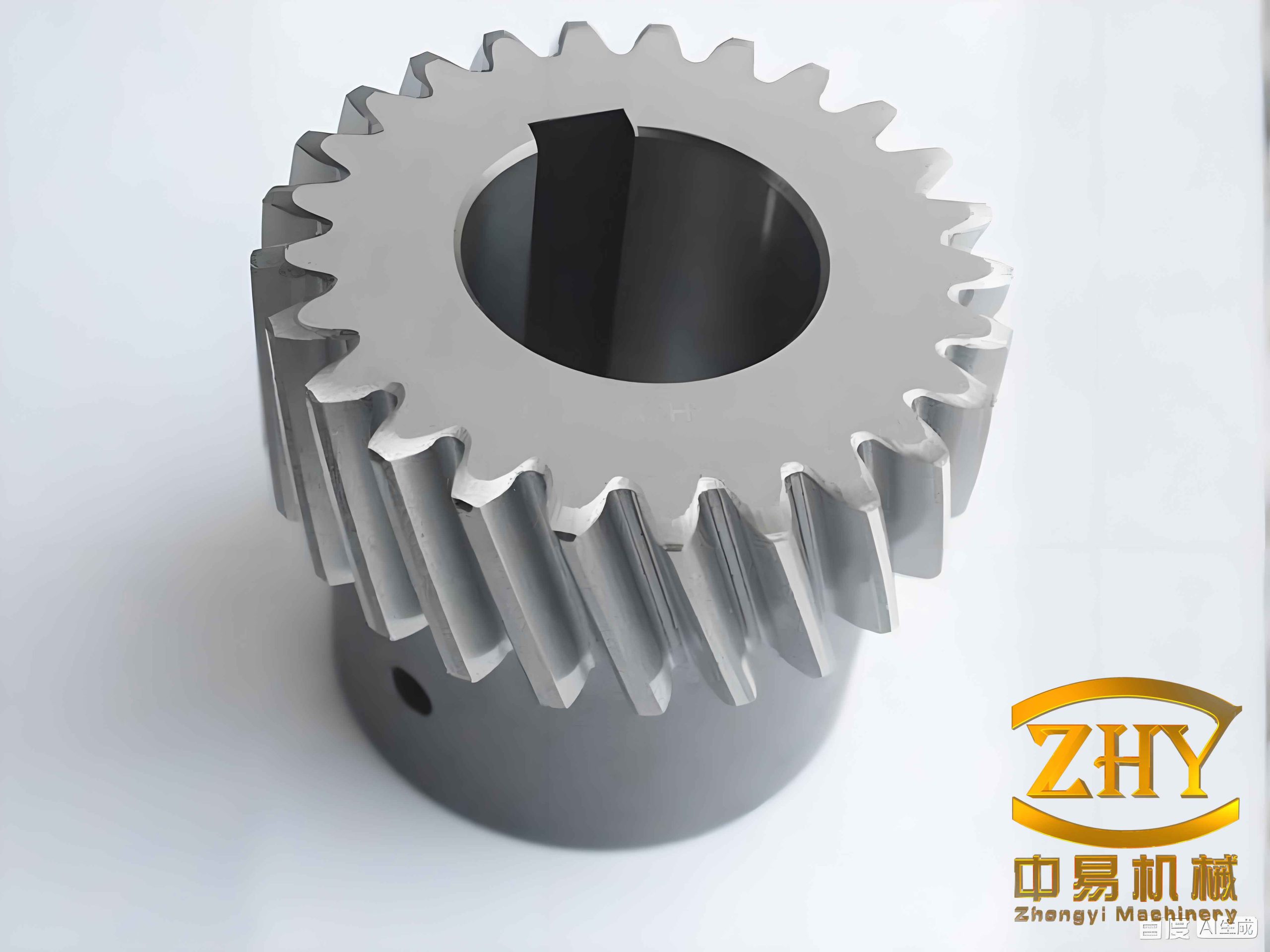
I have carried out a systematic study on the measurement of helical gear parameters using machine vision. Helical gears are widely used in industrial transmission systems because they offer smooth operation, high load capacity, and low noise. Compared with spur gears, helical gears have a helical angle, which makes their measurement more complex. Traditional measurement methods for helical gears are mostly contact-based, such as vernier calipers, micrometers, universal angle rulers, and coordinate measuring machines. These methods can achieve high accuracy, but they are slow, labor-intensive, and easily affected by human error. To overcome these limitations, I designed a machine vision based online measurement system for helical gears. The system uses multiple cameras to measure the addendum circle diameter, dedendum circle diameter, number of teeth, helical angle, and hand direction of helical gears. In this article, I describe the hardware selection, image preprocessing, edge extraction, parameter extraction, and error analysis. The experimental results show that the proposed method is fast and accurate, and it can meet the requirements of industrial online measurement.
Research Background and Significance
Helical gears are key components in vehicles, ships, machine tools, and aircraft transmission systems. The number of teeth has a great influence on the motion stability of helical gears. A helical gear with a large number of teeth generally runs more smoothly and is suitable for high-speed transmission. The helical angle of helical gears is not fixed, and different manufacturers often produce helical gears with different helical angles. A large helical angle is generally used in low-load scenarios, while a small helical angle is used in high-load scenarios. Therefore, accurate measurement of the helical angle is essential for the quality control of helical gears.
Machine vision has been widely used in industrial production because it is fast, non-contact, and non-destructive. However, many existing machine vision systems have problems such as too many measurement stations and tedious debugging. Each time a new type of workpiece is measured, the measurement system must be manually adjusted. In this research, I aimed to realize the online measurement of multiple parameters of helical gears, including addendum circle diameter, dedendum circle diameter, number of teeth, helical angle, and hand direction. I built an experimental platform that simulates an industrial production line. By fusing information from multiple cameras, I automatically adjusted the system parameters and improved the measurement speed and accuracy. To solve the problem of too many measurement stations, I integrated the measurement of multiple parameters into a single measurement station, saving space.
Measurement System Design
I designed a multi-camera machine vision measurement system for helical gears. The system consists of an upper camera for the end face and a side camera for the side surface. The upper camera measures the end face parameters, and the side camera measures the helical angle and hand direction. The system also includes light sources, lenses, a computer, and a graphical user interface. The measurement system is shown below.
For the end face measurement of helical gears, I used a front light source for close-range illumination to improve image contrast. Because helical gears have a special helical shape, backlight illumination cannot be used. I used edge continuation algorithms and Gaussian filtering algorithms to compensate for the influence of tooth surface defects on image processing. I also used the pinhole imaging principle to compensate for parallax and improve the measurement accuracy of the pixel equivalent. Different modules of helical gears were matched with different types of industrial lenses.
For the side measurement of helical gears, I built a side vision measurement system combined with the end face measurement system. I used a double telecentric lens camera to acquire side images of helical gears. I modeled and analyzed the tooth profile to verify the feasibility of the method. Then, I determined the hand direction by counting the number of specific structural elements. I used a Canny operator combined with a de-vignetting algorithm to extract edges. I used a morphology-based slope screening algorithm to process the edges and extract the tooth line edges. Finally, I measured the helical angle of the helical gears by curve fitting.
Camera and Lens Selection
The accuracy of a machine vision system depends on the camera resolution and lens distortion. A double telecentric lens has the advantages of wide depth of field, no perspective error within the working distance, and small distortion. It is widely used in machine vision measurement. However, compared with ordinary industrial lenses, double telecentric lenses have a smaller field of view, and large-field telecentric lenses are very expensive. When measuring small-module helical gears, it is best to use a double telecentric lens. When measuring large-module helical gears or considering cost, an ordinary industrial lens is preferred for measuring the end face parameters of helical gears.
I selected different cameras and lenses for different measurement tasks. The specifications are summarized in Table 1.
| Measurement Task | Camera | Lens | Resolution / Field of View |
|---|---|---|---|
| End face of large-module helical gears | CMOS camera | Ordinary industrial lens | 5496 × 3672 pixels, pixel size 2.4 μm × 2.4 μm |
| End face of small-module helical gears | CCD camera | Double telecentric lens | Depth of field 18 mm, field diameter 48 mm, actual field less than 40 mm |
| Side surface of helical gears | CCD camera | Double telecentric lens | Used for helical angle and hand direction measurement |
For large-module helical gears with a module greater than or equal to 1.25 mm, I used a high-resolution CMOS camera with an ordinary fixed-focus lens. For small-module helical gears with a module less than or equal to 1.25 mm, I used a double telecentric lens camera. The double telecentric lens avoids capturing the inner wall of the bore. In actual environments, mechanical vibration and assembly errors can cause eccentricity and tilt. An ordinary industrial camera produces both eccentricity error and perspective error, which further reduces measurement accuracy. A double telecentric lens can compensate for this error to some extent.
Because of mechanical incompatibility, the double telecentric measurement system could not be placed sideways in my design. I used an equivalent method to measure the side of the helical gears, which overcame the difficulty of mechanical incompatibility. I compared the measured image with the simulation result of the helical line of the helical gears, and the two matched perfectly. The effect of this method is the same as the theoretical value.
Light Source Selection and Assembly
Machine vision measurement generally requires high speed, and the camera exposure time is much shorter than that of an ordinary camera. This results in dark images and unclear details. Therefore, auxiliary lighting is usually needed. Light sources can be divided into invisible light and visible light. Ordinary industrial cameras generally use visible light for supplementary illumination. Common visible light sources include LED lamps, fluorescent lamps, and halogen lamps. LED lamps have a long life, fast response, and various colors, and they are suitable for most scenarios.
According to the illumination method, light sources can be divided into backlight sources, front light sources, structured light, and stroboscopic light sources. Backlight sources produce images with high contrast and are generally used for dimensional measurement. Front light sources are mainly used to detect surface details and defects, and they are easy to install. According to the illumination mode, light sources can be divided into dome lights, ring lights, shadowless lights, parallel lights, coaxial lights, point lights, low-angle lights, line lights, and gratings. A dome light is mainly used for defect detection of spherical or curved objects. Ring illumination is mostly used for surface quality inspection of smooth flat workpieces. A bar light is a light source that often illuminates from the side, and the commonly used angle is 45°. Side light can avoid strong reflection from frontal illumination and can also achieve bright illumination on edges, so it is often used for dimensional inspection. Coaxial light is used for metal, glass, and other highly reflective flat objects. It can enhance surface features with different angles, enhance surface texture, and reduce shadows. A shadowless light source is a light source whose light is diffusely reflected before illumination.
The illumination angle can be high angle, low angle, or multi-angle. High-angle illumination makes the overall image brighter and is suitable for objects with non-reflective surfaces. Low-angle illumination makes the background dark and the features white, which can highlight the contour and surface irregularities of the object. Multi-angle illumination makes the overall image softer and is suitable for curved objects.
For the end face of helical gears, I used a front light source installed close to the workpiece. For the side light source, I partially blocked a flat shadowless light source and used it as a bar light to slightly illuminate the side. Compared with spur gears, helical gears cannot use backlight illumination because of their special helical shape. Therefore, only front light sources can be used. This results in low contrast in the image, which brings great difficulties to machine vision measurement. To increase the contrast, the front light source should be installed close to the workpiece. Compared with a backlight source, a machine vision system using a front light source additionally captures redundant surface textures such as scratches, reflections, stains, and hair, which makes edge extraction more difficult. I proposed three solutions: first, clean the workpiece in advance; second, improve the image processing algorithm to highlight the required edges and suppress redundant edges; third, use a low-angle light source.
Other Components of the Measurement System
To fit the industrial production environment, the helical gear helical angle measurement system should be combined with the end face measurement system. An industrial device for online measurement of gear end faces can measure one gear every 2 seconds. My measurement system mainly includes a ring light source, a bar light source, a 2-megapixel CCD camera, a 20-megapixel CMOS camera, an ordinary industrial lens, a camera bracket, and a computer. I used two types of helical gears as examples: a 1.25 mm module, 25-tooth, 19° helical angle gear and a 1.5 mm module, 26-tooth, 45° helical angle gear. The shaft in the measurement system is only used to support the helical gears and is not used to rotate the workpiece. Theoretically, rotating the helical gears and using a 3D pseudo-reconstruction method can also measure the helical angle. However, I believe that the rotation measurement method has large errors and is slow, and it is difficult to apply to actual industrial production. Therefore, I did not use the rotation measurement method.
The computer used was a laptop with an AMD R7-5800H CPU. The CCD camera was fixed relative to the horizontal plane, and it needed to be centered and leveled in advance to collect side images of horizontally placed helical gears. The side camera required two spirit levels to adjust the pitch angle and the left-right tilt angle. I designed a graphical user interface to preview camera images and display measurement results.
Image Preprocessing
I first calibrated the camera, then performed distortion correction, ROI extraction, and grayscale conversion. The distortion in the center of the camera field of view is small. Collecting images when the workpiece passes through the center of the field of view can reduce measurement errors. In industrial vision measurement of gears, an automatic stopper is used to make the workpiece stationary in a fixed area. After the image is collected, the workpiece is released. Therefore, the horizontal coordinate of the ROI region is only related to the addendum circle diameter. When measuring helical gears with unknown parameters, the end face camera measures the addendum circle diameter, number of teeth, and pitch circle diameter. Without these parameters, it is impossible to perform curve fitting on the extracted tooth line edges.
Camera Calibration and Distortion Correction
I used the classic Zhang calibration method to calibrate the ordinary industrial camera. I selected an international chessboard calibration board and took more than 20 images from different directions. The purpose of camera calibration is to output the intrinsic parameters, extrinsic parameters, and distortion parameters. The further purpose is to determine the input-output relationship of the instrument or measurement system, determine the static characteristic index of the instrument or measurement system, and eliminate system errors. This calibration method does not require high precision for the calibration board images, but it has high requirements for the flatness of the calibration board. It is best to use a hard substrate such as ceramic or glass. The calibration of a double telecentric lens is slightly different from that of an ordinary industrial camera. I used a machine vision software to obtain the calibration parameters of the telecentric lens camera system.
Grayscale Conversion and Global Low-Illumination Enhancement
The ordinary industrial camera I used is a color camera. To simplify the image matrix, reduce the amount of computation, and improve measurement efficiency, I first converted the image to grayscale. Each pixel in a color image may be red, green, or blue. For an 8-bit image, the grayscale value of each pixel ranges from 0 to 255. A color image has 2^24 variations per pixel, which is too much information for image processing. Grayscale information is sufficient for image processing. Grayscale conversion simplifies computation and improves speed.
Considering the requirement of industrial measurement for image acquisition speed, I discussed image preprocessing under extremely short exposure time or weak light. The brightness of a photo is positively correlated with the exposure time. The shorter the exposure time, the darker the acquired image. Excessively increasing the exposure time will cause image blur and slow camera imaging. Therefore, global low-illumination enhancement is needed to simultaneously improve the brightness and contrast of the image. I used a global low-illumination enhancement algorithm. Because low-illumination images may lose details and reduce measurement accuracy, I used the global low-illumination enhancement algorithm only for image preview and debugging. In the subsequent binarization process, I could also choose to first perform global low-illumination enhancement and then use the Otsu binarization algorithm to achieve a similar effect.
ROI Extraction and Target Position Detection
ROI extraction algorithms can be divided into manual and automatic methods. Manual ROI extraction is often used when the ROI region of the image is constant. Common automatic ROI extraction methods include background subtraction, template matching, target tracking, and deep learning based matting algorithms. Automatic ROI extraction algorithms are often used in complex and changing scenes, such as real-time measurement for robotic arm grasping and autonomous driving. Due to the limitations of industrial production environments, it is difficult to ensure that the background is completely clean and tidy. Therefore, using background subtraction to extract the ROI region can be fast and effective. When the light changes little, background subtraction and optical flow methods are fast and effective.
Industrial light sources often have high power, high power consumption, and high heat generation. Long-term operation may cause overheating or aging. Therefore, vision measurement usually turns on the light source only when the workpiece moves under the camera. In most cases, the vision system is in a dark environment. To make the workpiece in the center of the image, the position of the workpiece must be known in advance by photoelectric measurement or visual detection. I used background subtraction to extract the ROI region. First, I subtracted the background image from the measurement image. Then, I binarized the background-subtracted image and removed small connected components. Finally, I determined the center position of the gear by the grayscale centroid method, which accumulates the coordinates of the points on the binary image and takes the average.
I compared several binarization algorithms, including Wellner, Niblack, Triangle, and Otsu. The two local binarization algorithms had poor results because the background subtraction did not completely eliminate the influence of the background. It is speculated that the brightness of the background in the two images changed slightly due to the reflection of the workpiece. When using local threshold algorithms, small grayscale changes are amplified. Global binarization algorithms can ignore these small grayscale changes, so they perform better. The Triangle algorithm is an adaptive threshold binarization algorithm, usually used for medical image segmentation, and is suitable for images with only a single grayscale peak. The Otsu algorithm is most suitable for images with two peaks in the grayscale histogram. The Otsu algorithm took 0.14 ms on my images. Considering both effect and speed, I used the Otsu algorithm as the binarization image segmentation algorithm for low-illumination images.
When there is no workpiece in the field of view, I should count the sum of grayscale values after binarization of the background image and set a grayscale threshold greater than this value. In this way, the system will not misidentify when the workpiece has not entered the camera field of view. After binarization, I found the coordinates of the grayscale centroid of the image, which is the approximate position of the workpiece. The addendum circle diameter of a gear is generally a negative tolerance. Using the upper camera to measure the actual addendum circle diameter can reduce the error of subsequent measurement results and also help automatically obtain the coordinates of the ROI region. The size of the ROI region can be obtained by first extracting the largest connected component of the binary image and then finding the minimum bounding rectangle. The side length of the rectangle is the preliminary measurement value of the addendum circle diameter.
Obtaining the Image Pixel Equivalent
The pixel equivalent of an image is the actual physical size represented by one pixel in the image. When measuring the pixel equivalent with a double telecentric lens camera, I used a standard 6×9 chessboard with each square measuring 6 mm × 6 mm. I used the Harris corner detection algorithm to detect corners. In actual measurement, twice the number of corners may be identified at one position, and a distance threshold is needed to identify adjacent corner coordinates. From the corner coordinates, the actual size represented by each pixel can be calculated. When the working distance changes little, the difference in pixel equivalent between the side and flat placement of the telecentric camera is small, and the precision requirement for the pixel equivalent on the side is not high. In my experiments, one pixel on the chessboard plane represented 0.0241 mm.
An ordinary industrial camera lens has perspective error. The closer the workpiece is to the camera, the larger the actual physical size represented by one pixel, and vice versa. Therefore, to obtain an accurate pixel equivalent, the height of the workpiece end face must be measured by a side-mounted telecentric camera. Under different distances from the camera, the ratio of the image size to the object distance follows the relation:
$$ \frac{u_1}{u_2} = \frac{w_1}{w_2} $$
where \(u_1\) and \(u_2\) are different image distances, and \(w_1\) and \(w_2\) are different object distances. When the focal length is not changed, the image distance of the camera is a fixed value. The ratio of the pixel size under different object distances is:
$$ \frac{w_1}{w_2} $$
The object distance of my industrial camera is much larger than twice the image distance. Therefore, according to the lens imaging principle, the CMOS should form an inverted reduced real image, and the image distance is between one and two times the focal length. In the case of no focus change, the perspective error is shown in the following relation. For a pinhole imaging model, focusing is achieved by changing the distance between the lens and the image plane, that is, the image distance, so that the image plane falls within the depth of field. The intrinsic and extrinsic parameters of the camera also change. When focusing on a near object, the field angle becomes smaller.
When measuring the pixel equivalent of the end face image, I measured the pixel equivalent of the same edge length of a gauge block with a nominal size of 20 mm (±2 μm) in both standing and lying states to verify the parallax formula. The gauge block had a length of 35 mm, a width of 20 mm, and a thickness of 9 mm. The distance from the camera when the gauge block was lying flat was 26 mm greater than when it was standing. The relationship between the true object distance and the pixel equivalents is:
$$ \frac{pix_s}{pix_l} = \frac{w + 26}{w} $$
where \(pix_s\) is the pixel equivalent of the measured plane when the gauge block is standing, and \(pix_l\) is the pixel equivalent of the measured plane when the gauge block is lying down. From the true object distance obtained by the formula, the pixel equivalent at other heights can be calculated. Because a telecentric lens has no perspective error, the pixel equivalent can be measured with a gauge block within the working range of the telecentric lens. Within the working range of the telecentric lens, the pixel equivalent does not change significantly with the size of the helical gear or the distance from the telecentric camera.
I used the subpixel edge detection algorithm to measure the pixel equivalent with a gauge block. The two lenses used the same 20-megapixel CMOS sensor. The pixel equivalents measured for several helical gears are shown in Table 2.
| Lens Type and Workpiece Height | Pixel Equivalent | Lens Type and Workpiece Height | Pixel Equivalent |
|---|---|---|---|
| Double telecentric lens, 9 mm | 24.13 μm | Ordinary industrial lens 1, 20 mm | 13.58 μm |
| Double telecentric lens, 9 mm | 24.13 μm | Ordinary industrial lens 2, 20 mm | 38.02 μm |
From Table 2, the pixel size of ordinary industrial lens 2 is much larger than that of ordinary industrial lens 1 because the working distance and field of view of lens 2 are larger than those of lens 1. With the same hardware, moving the lens closer to the workpiece can reduce the pixel equivalent and improve measurement accuracy. Compared with the method of measuring the pixel equivalent using a calibration board, using a gauge block is more stable. The measurement accuracy using a gauge block is lower than that of a ceramic calibration board but higher than that of a plastic calibration board. The calibration board method is greatly affected by the flatness and tilt angle of the calibration board. Moreover, the calibration board occupies a large area and cannot always be placed in the camera field of view. The gauge block can be placed in the measurement system at any time to correct the pixel equivalent, which is conducive to realizing the automation of the measurement system. To improve the stability and automation of the measurement, the end face measurement system used a gauge block to measure the pixel equivalent.
Edge Extraction of Helical Gear Images
Edge extraction technology is an important application of image segmentation. Classical edge extraction technologies include Canny, Sobel, and Laplace algorithms based on gradients. Deep learning based edge detection algorithms include HED and Deeplab. Deep learning based edge extraction algorithms have good edge detection results for complex images, but they are slow and not suitable for small sample datasets. The HED algorithm takes about 14 s. Traditional gradient-based edge detection algorithms usually run in tens of milliseconds. Industrial measurement requires high speed, and ideal measurement environments such as darkrooms can be built manually. Therefore, industrial measurement generally uses traditional edge detection operators. Different image filtering algorithms have different effects on edge extraction. Therefore, I discussed image filtering and edge extraction together and separated the edge extraction of the end face and side images.
Filtering and Edge Extraction of the End Face Image
In machine vision measurement, there may be multiple measurement stations, so multiple light sources are needed for illumination. The light from multiple sources and reflected light can make the image brightness uneven and increase the difficulty of image processing. Filtering algorithms for uneven image brightness include homomorphic filtering, de-vignetting algorithms based on maximum and minimum filtering, de-vignetting algorithms based on entropy, and brightness correction algorithms based on gamma functions and light distribution characteristics.
The end face of a gear is generally a plane parallel to the light source. It has a strong ability to reflect light and has high contrast with the background. Unlike spur gears, part of the side profile of helical gears is also captured by the end face camera. This part of the surface is inclined, and its brightness is slightly higher than the background brightness. Compared with the edge extraction of the end face of spur gears, the requirement for threshold accuracy is higher. I processed the end face image with Gaussian filtering. The results showed that Gaussian filtering greatly weakened the texture in the image, while the influence on the workpiece contour was small. The end face contour of helical gears with a blackened surface has low contrast, so it is best to measure before the workpiece undergoes surface blackening treatment. Compared with several classical edge-preserving filtering algorithms, Gaussian blur had a better effect, mainly because the image gradient of the surface texture in my images was strong. Edge-preserving filtering could hardly screen out the true edges in these images.
Subpixel edge detection algorithms greatly improve the measurement accuracy of end face parameters. Therefore, I used a subpixel edge extraction algorithm for end face edge extraction. Although subpixel edge detection has higher accuracy than pixel-level edge detection, its speed and difficulty of data analysis are higher. I used pixel-level edge detection to measure parameters with low requirements on edge detection accuracy, such as the number of teeth. I used subpixel edge detection to measure parameters with high requirements on edge extraction accuracy, such as the addendum circle diameter and dedendum circle diameter.
The Canny algorithm has the advantages of high positioning accuracy, high signal-to-noise ratio, and single-edge response, and it has been widely used. The traditional Canny edge detection algorithm requires manual setting of high and low thresholds according to the specific conditions of the detected image. In practical applications, the trial-and-error method is usually used to continuously adjust the high and low thresholds until an ideal edge image is obtained. Once the measured object or environment changes, the parameters need to be readjusted. This method is inefficient and difficult to realize automatic real-time detection. The Otsu algorithm is also called the maximum between-class variance method. The adaptive Canny algorithm combined with Otsu is a classic adaptive edge detection algorithm. The Otsu algorithm divides the image into background and foreground according to the grayscale characteristics of the image. The greater the variance between the two classes, the greater the difference between the foreground and the background. When a threshold maximizes the variance between the two classes, the threshold is the optimal segmentation threshold. The Otsu algorithm itself is a classic image segmentation algorithm. Applying the idea of Otsu to Canny can adaptively select the high and low thresholds of the Canny algorithm. The adaptive Canny combined with Otsu is mostly used for relatively simple images. For complex images, the effect of this algorithm is not excellent. Different algorithms should be used for different images to achieve the best edge segmentation effect. My Canny edge detection algorithms were all used together with Gaussian filtering. According to the actual situation, I used the Otsu adaptive Canny operator to extract the contour edge of the helical gear end face.
After edge detection, I filled holes in the image. However, due to the influence of metal debris, the extracted edge may have breakpoints, which prevents the next step from successfully filling the holes. Therefore, I connected the tooth edge, which is also called edge closing. The bwmorph function can connect adjacent breakpoints in the eight-neighborhood, but if the breakpoints are not in the same eight-neighborhood, they cannot be connected, and mismatches may occur. In image processing, a breakpoint can also be called an endpoint of a connected component. An endpoint can be understood as a pixel connected to only one pixel. Sometimes the edge obtained by Canny edge detection has a width of more than one pixel. My method first thinned the edge, then found the endpoints, recorded the coordinates of the endpoints, and set a distance threshold. If the distance was within this threshold, the two pixels were connected to complete the connection of the breakpoints. By traversing the image, I found the pixel coordinates that were connected to only one point in the eight-neighborhood, that is, whether the number of pixels in the eight-neighborhood of this point was 2. Then I used the DDA line drawing algorithm to connect the endpoints.
Filtering and Edge Extraction of the Side Image
According to the characteristics of the helical gear side image, the following filtering algorithms may have optimization effects: DCT denoising, HDR, Gaussian filtering, de-vignetting, homomorphic filtering, high-pass preservation, edge-preserving sharpening, and low-pass filtering. After experimental comparison, the de-vignetting algorithm had the best effect under my conditions.
DCT denoising is also called discrete cosine transform denoising, which is generally used to remove salt-and-pepper noise. HDR stands for High Dynamic Range. The dynamic range of an image refers to the ratio of the maximum to the minimum brightness value. The larger the dynamic range, the more details the image displays and the more realistic the visual effect. The HDR algorithm I used was Hyper-HDR, whose purpose is to clearly record image details under a light source. HDR has become an important part of computational photography. Gaussian filtering is essentially a weighted average blurring algorithm. The grayscale value of each point is obtained by weighted averaging of itself and other pixel values in its neighborhood. Gaussian filtering is very effective for removing impulse noise. Vignetting is a photography term that refers to the decrease in brightness or saturation at the periphery compared with the center of an image. The four corners of the image become darker. The de-vignetting algorithm is a special shadow correction algorithm. The entropy-based de-vignetting algorithm minimizes the entropy of the entire image and can effectively correct shadows. Homomorphic filtering was proposed in the 1960s and is a method that simultaneously compresses the brightness range and enhances the contrast of an image in the frequency domain. The high-pass preservation algorithm retains the pixels in the image that have a large contrast with the surrounding area, and all other parts become gray. The core calculation of the high-pass preservation algorithm can be summarized as subtracting the Gaussian blurred image from the original image and then performing global brightness enhancement. The low-pass filtering algorithm can smooth the image and filter out noise. The edges and grain noise of an image are high-frequency components, and the background is often a low-frequency component. Filtering out the high-frequency part achieves the purpose of removing noise. In the image of the helical gear side surface, the contour edge has the highest frequency, followed by noise points. Therefore, using a low-pass filter in some cases can retain only the contour edge information.
For smaller-module helical gears, the illumination change on the side is more obvious. Under natural light, I took a 1.25 mm module, 25-tooth, 19° helical angle helical gear as an example. The results of various image filtering algorithms are compared. The DCT denoising, HDR, Gaussian filtering, de-vignetting, high-pass preservation, homomorphic filtering, edge-preserving sharpening, and low-pass filtering all have their own advantages and disadvantages. The de-vignetting algorithm achieved the best balance between illumination compensation and edge preservation.
From the side image, it can be seen that under darkroom conditions, due to the special tooth shape of helical gears, the brightness and contrast of the gear surface are extremely uneven. For a left-handed helical gear illuminated by an upper light source, the left and right edges of the image are clear, and the illumination intensity is high on the left and top and low on the right and bottom. A right-handed helical gear is the opposite. This makes the contrast at the gear center and the right position too low, which is unfavorable for edge extraction.
Ant colony optimization is a bionic intelligent algorithm, similar to deep learning based edge detection algorithms. The edges obtained by intelligent algorithms are generally thick and not suitable for high-precision machine vision measurement. However, intelligent edge detection algorithms often perform better than traditional gradient-based edge detection algorithms for complex images. The edge detection of the ant colony algorithm regards edge detection as a process of clustering pixels with different features. Each pixel is regarded as an ant, and each ant is a three-dimensional vector characterized by grayscale, gradient, and neighborhood. The Sobel operator and Canny operator are the most classic edge detection algorithms. The Sobel operator uses the weighted difference of the grayscale values of the four neighborhoods of each pixel in the image. The edge is detected when the extreme value is reached. The Sobel algorithm can detect horizontal or vertical edges separately. The Canny algorithm has a high edge detection rate, and the detected edges have fewer breakpoints, but it is easy to mark noise as edge points.
The regional edge detection algorithm divides the image into several segments and sets edge detection thresholds separately. The side image of a helical gear can be divided into left, middle, and right parts. The gradient values of the left and right parts are obviously different from those of the middle part. Performing edge detection on the image by region can reduce the false edge detection rate of the middle part and improve the detection rate of weak edges in the left and right parts. After edge detection on the three images separately, the images can be spliced to obtain the edge detection image of the whole image. Unlike other image stitching algorithms, the image stitching algorithm used here is the simplest matrix stitching algorithm, which can only stitch matrices with the same number of rows, and the computational complexity is on the same order as matrix addition and subtraction. In particular, shearing destroys the original eight-neighborhood at the edge, and the results of edge detection operators at the image edge are inaccurate. When shearing the image, at least 2 more rows should be cut (10 rows in my case), and then the extra columns should be removed during image stitching.
I compared the edge extraction effects of different algorithms. The Sobel operator without filtering and the Canny operator combined with a high-pass filter detected edges with many obvious breakpoints. The Canny operator combined with phase consistency had almost the same effect as the Canny operator using a Gaussian filter. The Canny operator combined with the HDR algorithm had an effect similar to grayscale equalization in weak light areas, but the edge detection effect in other areas became worse. The edges detected by the ant colony algorithm were smooth, but the problem of breakpoints was not solved. Under global threshold conditions, the above edge detection methods all had poor results. For the regional edge detection algorithm, only the middle part of the image could use adaptive threshold Canny. The Gaussian filter kernel and edge detection threshold of the left and right parts needed to be set manually. The reflection from the tooth bottom was mistakenly identified as an edge when using the Otsu adaptive threshold.
In the early stage, I thought homomorphic filtering had the best effect. After introducing the entropy-based de-vignetting algorithm and the edge-preserving sharpening algorithm, I found that the de-vignetting algorithm was better than homomorphic filtering in optimizing uneven illumination. The edge-preserving sharpening algorithm can improve the strength of edges, thereby improving the effect of edge detection. The de-vignetting algorithm is a newer illumination compensation algorithm. Compared with homomorphic filtering, it is less difficult to debug and has a better effect. The side image of helical gears is similar to a vignetting image. A vignetting image is an image in which the brightness of the four corners is obviously darker. Vignetting is also called light falloff. Vignetting is common in images taken with wide-angle lenses.
I used a de-vignetting algorithm based on the minimization of log-intensity entropy. Its core theory is to minimize the entropy of the entire image. Ordinary entropy encounters local optimal problems during optimization, and the concept of logarithmic entropy can solve this problem. Suppose the histogram of a normal image is a single peak distribution. If the image has vignetting, its histogram will have another low-brightness distribution. The process of correcting vignetting is to move the low-brightness distribution closer to the original normal brightness.
Morphological Processing of Edge Images
Mathematical morphology is an image processing method based on set theory and algebra. It is usually applied in the image processing part after edge detection. It can compensate for the shortcomings of edge detection and reduce image noise. Common morphological image processing algorithms include erosion and dilation algorithms and hit-or-miss algorithms. Erosion and dilation algorithms are often used to remove burrs on the edges of binary images and separate connected components.
From the shape of the tooth line, slope screening is the most reliable method for edge selection. The hit-or-miss transform is an important morphological algorithm. I used an improved hit-or-miss transform algorithm to implement slope screening and extract the required tooth line edges. The improved hit-or-miss transform algorithm has the following steps. First, I constructed structural elements, traversed the image, cleared the parts identical to the structural elements, and retained the parts that were not identical. This can break redundant edges connected to the tooth edge. By changing the structural elements, unnecessary horizontal and vertical lines in the image can be removed, and only the tooth line edge parts are retained. The morphological processing flow includes several key steps, and the structural elements are defined as follows:
$$ S_1 = \begin{bmatrix} 0 & 1 & 1 \\ 1 & 0 & 0 \\ 1 & 0 & 0 \end{bmatrix}, \quad
S_2 = \begin{bmatrix} 1 & 1 & 0 \\ 0 & 0 & 1 \\ 0 & 0 & 1 \end{bmatrix}, \quad
S_3 = \begin{bmatrix} 1 & 1 & 1 \\ 1 & 1 & 1 \end{bmatrix} $$
where \(S_1\) is the +45° slope structural element, \(S_2\) is the -45° slope structural element, and \(S_3\) is the horizontal structural element. The morphological algorithm had a good compensation effect on the defects of edge extraction.
Extraction of Helical Gear Parameters
The end face parameters of a gear mainly include addendum circle diameter \(d_a\), pitch circle diameter \(d\), number of teeth \(z\), bore diameter, base circle diameter \(d_b\), dedendum circle diameter \(d_f\), module \(m\), pitch \(p\), and tooth height \(h\). The processing of standard cylindrical gears requires at least three parameters: module, number of teeth, and bore diameter. To simplify the calculation, my measurement data were expressed in pixel units before the final output. When outputting the measurement results, the pixel size is multiplied by the pixel equivalent to obtain the actual physical size of the helical gear parameters.
Preliminary Measurement of Addendum and Dedendum Circle Diameters
The addendum circle diameter \(d_a\) is the diameter of the circle where the addendum edge of a cylindrical helical gear is located. For an external gear, the addendum circle diameter is the largest circle on the gear. Circle detection algorithms are a common method for detecting the addendum circle edge. Classic circle detection algorithms include the least squares circle fitting algorithm, Hough transform circle detection algorithm, maximum enclosing circle algorithm, and minimum enclosing circle algorithm. I performed preliminary measurements of the addendum and dedendum circle diameters, allowing a certain error.
For the measurement of the addendum circle diameter based on the minimum enclosing circle algorithm, I analyzed that it is not necessary to use a circle detection algorithm. After background subtraction and removal of small connected components, the image except for the workpiece is pure background. In this case, the outer contour of the image, that is, the tooth edge where the addendum circle is located, can be found by traversing the image. This method can remove the inner bore edge and keyway edge, avoiding interference with the measurement and analysis of gear tooth parameters such as the addendum circle diameter. First, I used a boundary tracking algorithm to obtain the edge image of the outer contour of the helical gear workpiece. Then I filled the holes in the binary image of the gear outer contour edge and calculated the average distance between the center and each point to obtain the approximate diameter of the addendum circle. I used the Euclidean distance. Let the coordinates of the edge point be \(G(i,j)\). The calculation formula for the gear center coordinates is:
$$ x_c = \frac{\sum x_i}{i}, \quad y_c = \frac{\sum y_i}{i} $$
where \(i\) is the number of pixels, \(x_i\) and \(y_i\) are the horizontal and vertical coordinates of the \(i\)-th pixel, and \(x_c\) and \(y_c\) are the coordinates of the geometric center of the gear. The calculation formula for the addendum circle diameter is:
$$ d_a = \frac{2 \sum \sqrt{(x_i)^2 + (y_i)^2}}{i} $$
The double telecentric lens can measure the addendum circle using the same method as an ordinary camera, or it can use a backlight source. When using a backlight source, the gear contour is approximately a standard circle. The minimum enclosing circle algorithm can obtain the addendum circle diameter. The pixel-level measurement method of the dedendum circle is similar to that of the addendum circle, using the maximum inscribed circle algorithm.
I also discussed a method for measuring the addendum circle diameter by finding the peak of a vector. I counted the number of pixels within a certain distance from the gear geometric center and used this number as the value of the vector element. This method is similar to building a grayscale histogram. Pixels with the same pixel distance from the gear geometric center (within 1 pix/10) were grouped into one class. A line chart was drawn with the number of pixels in each equal pixel distance as the x-axis. The distance between the edge point and the gear center corresponding to this edge point can be used as a basis for screening the addendum circle part and the tooth part in the outer contour edge. Theoretically, this method can improve the measurement accuracy of the addendum circle diameter to the subpixel level. The actual measured error of the addendum circle diameter was only 1.3 pix, and the error of the dedendum circle diameter was 2.4 pix, which is comparable to the accuracy of the minimum enclosing circle algorithm. The positioning error of the gear geometric center based on pixel-level edge detection has a great influence on this algorithm. The signal processing of this method is complex, and the same parameters are difficult to produce the same optimization effect on different data. It did not achieve adaptive adjustment and may require optimization by intelligent algorithms such as SVM. I only used it as a comparison and outlook.
Measurement of the Number of Teeth
There are several methods for measuring the number of teeth of helical gears. Previous research has achieved good recognition results for spur gears. There are mainly three methods. One method is to measure the addendum and dedendum circle diameters, calculate the diameter interval where the tooth profile of the gear is located, thin the edge, and then expand the edge image of the gear into a rectangle with the gear center as the center. In this way, the number of teeth can be calculated by counting the number of points when the vertical coordinate is the pitch circle diameter. This method is easily affected by surface defects of the gear. Another method is to detect the number of teeth based on the connected components of the binary image. I call this method the statistical connected component method. The third method is to draw a circle with the middle value of the addendum and dedendum circle diameters after knowing the diameters, calculate the number of intersections between this circle and the tooth edge, and calculate the distance between each intersection. In the absence of abnormal points, the distances between the points are almost the same. Sometimes, the surface of helical gears may have cutting debris, hair, clothing fibers, dust, and other contaminants. These contaminants can destroy the normal contour of the helical gear image. Using a threshold algorithm to remove singular points, half of the number of intersections is the number of teeth.
The statistical connected component method is more stable and robust for detecting the number of teeth of helical gears. Therefore, I used the connected component method to measure the number of teeth. After preliminarily obtaining the dedendum and addendum circle diameters of the helical gear, I drew a circular mask with the average of the two diameters as the diameter, multiplied the mask by the binary image, and extracted the tooth part of the helical gear end face image. Then I calculated the number of teeth using the statistical connected component method. To avoid the influence of edge defects, I also performed erosion on the connected components. After measuring the number of teeth, I calculated the centroid coordinates of each connected component. These centroids participated in the classification of subpixel points in the following steps.
Subpixel Measurement of the Addendum Circle Diameter
Subpixel edge extraction technology subdivides the basic unit of pixels in an image and can improve the accuracy of edge detection to a certain extent without changing the hardware conditions. The edges detected by subpixel edge detection cannot be composed of isolated points but must be multiple pixel points with a certain distribution pattern. Current subpixel edge detection algorithms can be summarized into three types: fitting methods, moment methods, and interpolation methods. I used a subpixel edge detection algorithm based on partial area effect, which has high speed and accuracy.
The core idea of subpixel edge detection is to assume that the edge is discontinuous in the intensity function \(F\). When the edge passes through a single pixel \((i, j)\), the pixel intensity is expressed as:
$$ I_{i,j} = \frac{A S_A + B S_B}{h^2} = B + \frac{A – B}{h^2} P_{i,j} $$
where \(A\) and \(B\) are the intensities on both sides of the edge, \(S_A\) and \(S_B\) are the areas corresponding to the different intensities \(A\) and \(B\) in the pixel, \(h\) is the side length of a single pixel, and \(h^2 = S_A + S_B\). Here \(h = 1\). A straight edge with a slope between 0 and 1 is represented by the equation \(y = a + bx\). Consider a 5×3 pixel window with the middle pixel at \((i, j)\). The expressions for the pixel areas of the left, middle, and right columns are represented by \(L\), \(M\), and \(R\). From the expression for \(M\), the coefficient \(a\) can be obtained as:
$$ a = \frac{S_M (A – B) + h^2 (A + B)}{2(A – B)} – \frac{h}{2} $$
The coefficients \(a\) and \(b\) are:
$$ b = \frac{2(S_R – S_L)}{A – B} $$
The subpixel position is \((0, a)\) in the coordinate system with the center of the pixel \((i, j)\) as the origin, that is, the point at a distance of \(a\) pixels from the pixel center in the positive y direction. The normal vector from the pixel center \((i, j)\) to the edge line is:
$$ \mathbf{n} = \frac{A – B}{\sqrt{1 + b^2}} \begin{bmatrix} -b \\ 1 \end{bmatrix} $$
I used the nearest-neighbor interpolation algorithm to super-resolve the grayscale image of the original image, and then overlapped the subpixel edge obtained by subpixel edge detection with the normal vector on the super-resolved image. Common image analysis methods for measuring the dedendum circle diameter include the minimum inscribed circle method, which is easily affected by abnormal points. The tooth image of a helical gear shows that the overlapping part of the addendum circle and the end face contour of the gear is several discrete arcs. Extracting points on these discrete arcs is the key to measuring the dedendum circle diameter.
The subpixel measurement process of the addendum and dedendum circles includes the following steps. First, I calculated the angle of the line connecting the centroid of each connected component obtained in the tooth number measurement and the geometric center of the gear. The size of each angle is approximately \(\pi/z\). I used these angles to classify the tooth edge coordinates obtained by subpixel edge detection. I calculated the minimum distance from each region to the gear geometric center. In this way, each subpixel coordinate of the dedendum can participate in the calculation of the dedendum circle diameter. The calculation of the addendum circle is similar to that of the dedendum circle. I rotated the angle partition of the addendum circle by \(\pi/z\) around the gear geometric center so that each partition could completely include an addendum region. I recorded the point with the farthest distance from the gear center in each region.
The slope of the edge point relative to the gear geometric center is:
$$ k_{i,j} = \frac{y_i – y_c}{x_i – x_c} $$
where \(k_{i,j}\) is the slope of the line connecting the pixel point with image coordinates \((i,j)\) and the gear geometric center. The angles of the lines connecting the centroids of two adjacent connected components and the gear geometric center were used to classify edge points. A pixel point with \(k_{i,j}\) in the region between two adjacent angle regions, that is, a sector region, forms a complete edge of a tooth. After obtaining the above coordinates, I used the least squares circle fitting algorithm to process the addendum and dedendum circle coordinates separately to obtain the diameters of the addendum and dedendum circles. I used the \(3\sigma\) rule in the normal distribution to remove outliers and took the result of the second fitting after removing outliers as the final result. Because the number of sampling points in a single measurement exceeded 10, and the deviation between the distance of each point from the circle center and the fitted circle radius followed a normal distribution, the \(3\sigma\) rule was effective.
For a 1.25 mm module, 25-tooth, 19° helical angle helical gear, the measured pixel radii of the addendum and dedendum circles were 1312.8 pix and 1104.35 pix, respectively. After multiplying by the pixel equivalent, the actual physical dimensions of the addendum and dedendum circle diameters were 35.65564 mm and 29.9941 mm, with errors of 4.4 μm and 9.4 μm compared with the design values. When using the double telecentric lens camera to measure the addendum circle diameter, the error was 10.81 μm, which is less accurate than the ordinary lens camera measurement system. The main reason is that the double telecentric lens is matched with a 2-megapixel camera with a small sensor size. The sensor size of the 20-megapixel CMOS is too large and does not match the double telecentric lens.
Obtaining the Pitch Circle Diameter and Base Circle Diameter
The module and number of teeth can be used to derive the addendum circle diameter, pitch circle diameter, base circle diameter, and other parameters. The relationship between the dedendum circle diameter, pitch circle diameter, and module is:
$$ d_f = d – 2.5m $$
For standard cylindrical helical gears, the relationship between the addendum circle diameter, pitch circle diameter, and module is:
$$ d_a = d + 2m $$
The pitch circle diameter \(d\) is the basis for calculating the dimensions of various parts of the gear. On the pitch circle of a standard gear, the tooth thickness and tooth space width are equal. The pitch circle diameter is equal to the module multiplied by the number of teeth. The standard cylindrical helical gear pressure angle \(\alpha\) is generally 20°. The relationship between the base circle diameter and the pitch circle diameter is:
$$ d_b = d \cos(\alpha) $$
The addendum part of a general helical gear is polished or cut, so the addendum circle diameter is different from that of a standard gear. Therefore, it is more reliable to calculate the pitch circle diameter based on the dedendum circle diameter. The module is obtained in advance from the technical specifications.
Extraction of Side Parameters of Helical Gears
The side parameters of helical gears mainly refer to the hand direction and the helical angle. The non-contact measurement methods for the helical angle of helical gears mainly include laser measurement, structured light method, and machine vision method. A helical gear is a cylindrical gear with helical teeth. The tooth line is a collection of helical lines on the side of the helical gear. The parametric equation of a helical line in a spatial rectangular coordinate system is:
$$ x = r \cos\left( \frac{2(n-1)\pi}{c} + \theta_0 \right) $$
$$ y = r \sin\left( \frac{2(n-1)\pi}{c} + \theta_0 \right) $$
$$ z = r \cot(\beta) \theta = \pm \frac{r}{\tan(\beta)} \theta $$
where \(c\) is the number of teeth of the helical gear, \(n\) is an arithmetic sequence from 1 to \(c\) with a step of 1, \(\theta\) is the angle parameter, \(\beta\) is the helical angle of the helical gear, and \(z\) is the z-axis coordinate. In the end face coordinate system, the rotation angle of the helical line corresponding to each tooth is \(2\pi/c\) radians. When the sign of \(r\) and \(b\) is negative, the helical gear is left-handed; otherwise, it is right-handed.
Taking a 1.5 mm module, 26-tooth, 15 mm thick, 45° helical angle helical gear as an example, I substituted the parameters into the formula and obtained the three-dimensional schematic diagram of the gear tooth shape. The projection of the helical line on the xoz plane is not a straight line, but the projection of the middle tooth line is approximately a straight line. Because the camera can only capture the front image of the gear, the tooth profile curve in the \(y > 0\) part is invisible. Therefore, \(0 < 2(n-1)\pi/c + \theta_0 < \pi\). I only considered the tooth profile part that the camera can capture.
By combining the formulas, the function expression of \(x\) and \(z\) can be obtained:
$$ z = z_0 + \frac{(x – x_0) \tan(\beta)}{r} \left( \frac{2(n-1)\pi}{c} + \theta_0 \right) $$
With other parameters unchanged, I changed the value of \(\beta\) within a certain range. The projected curves had uniqueness, and no curve coincided with another. Their shapes were completely different. The theoretical error of the direct line method compared with my curve fitting method is about 0.91% for a 1.5 mm module, 26-tooth, 45° helical gear. Under ideal conditions, the error of my algorithm depends only on the camera resolution and the errors of parameters such as the addendum circle diameter obtained from the end face vision measurement. For helical gears with a helical angle less than 10° and a thickness less than 10 mm, the theoretical error of the straight-line measurement algorithm is extremely small, and the previous algorithm is simpler and faster.
The conversion relationship between the addendum circle helical angle and the pitch circle helical angle is:
$$ \tan(\beta) = \frac{P}{\pi d} $$
$$ \tan(\beta_y) = \frac{P}{\pi d_y} $$
where \(P\) is the lead of the helical surface, which is constant, and \(d_y\) is the addendum circle diameter. The pitch circle helical angle \(\beta\) is:
$$ \beta = \arctan\left( \frac{d}{d_y} \tan(\beta_y) \right) $$
Determination of the Hand Direction of Helical Gears
Helical gears are divided into left-handed and right-handed. For an external gear, when viewed from bottom to top, if the helical line advances from the lower right to the upper left, it is a left-handed helical gear; otherwise, it is a right-handed helical gear. Different hand directions of helical gears and the same hand direction of helical gears have different transmission modes, which are divided into crossed-axis and parallel-axis transmission. The significance of measuring the hand direction is to determine the sign of \(r\) and \(b\). I first removed connected components with too small an area from the Canny edge image of the ROI image. Then I traversed the edge image and found the numbers of structural element 1 and structural element 2. According to the numbers of structural elements, I determined whether the gear was left-handed or right-handed.
The structural elements I used are:
$$ S_1 = \begin{bmatrix} 0 & 1 \\ 1 & 0 \end{bmatrix}, \quad
S_2 = \begin{bmatrix} 1 & 0 \\ 0 & 1 \end{bmatrix}, \quad
S_3 = \begin{bmatrix} 1 & 0 & 0 \\ 0 & 1 & 0 \\ 0 & 0 & 1 \end{bmatrix}, \quad
S_4 = \begin{bmatrix} 0 & 0 & 1 \\ 0 & 1 & 0 \\ 1 & 0 & 0 \end{bmatrix}, \quad
S_5 = \begin{bmatrix} 1 & 1 & 1 & 1 \end{bmatrix} $$
where \(S_1\) is the +45° slope structural element, \(S_2\) is the -45° slope structural element, and \(S_5\) is the horizontal structural element. Because of chamfering, the specifications of several gears used in this section are shown in Table 3.
| Gear Number | Module (mm) | Number of Teeth | Helical Angle (°) | Hand Direction | Type |
|---|---|---|---|---|---|
| Z-1# | 1.5 | 26 | 45 | Right | Helical gear |
| Z-2# | 1.5 | 22 | 19 | Left | Helical gear |
| Z-3# | 2 | 30 | 19 | Left | Helical gear |
| Z-4# | 1.5 | 30 | 19 | Left | Helical gear |
| Z-5# | 1.25 | 25 | None | None | Spur gear |
The texture slope on the side image of a left-handed helical gear is mostly negative, while that of a right-handed helical gear is mostly positive. This algorithm is greatly affected by noise, so the image needs to be Gaussian filtered in advance. The numbers of structural elements in the edge images of several helical gears are shown in Table 4.
| Structural Element | Z-1# | Z-2# | Z-3# | Z-4# | Z-5# (-1°) | Z-5# (+5°) |
|---|---|---|---|---|---|---|
| 1 | 28861 | 1569 | 2270 | 443 | 934 | 917 |
| 2 | 11946 | 2637 | 3988 | 1004 | 3242 | 872 |
From Table 4, helical gears with different hand directions have great differences in the numbers of the two structural elements. Under extreme conditions such as a helical angle of 19° to 45° and overexposure, the accuracy of the algorithm is not affected. Because spur gears are affected by irregular specular reflections, this method cannot determine whether a gear is a spur gear. This algorithm took 27.3 ms on a 781×1558 ROI image.
Curve Fitting of Edge Lines
I fitted the curve in a plane rectangular coordinate system. I transformed the horizontal and vertical coordinates of the points on an extracted edge to a coordinate system with the workpiece axis as the y-axis and the upper end face of the gear image as the x-axis, and compensated for the workpiece tilt angle. Because the image coordinate system is opposite to the plane rectangular coordinate system, the coordinate \((y_0, x_0)\) corresponding to the origin of the coordinate system in the image is \((x_0, y_0)\) in the plane rectangular coordinate system. The coordinate relationship when the workpiece is not tilted is:
$$ x_{real1} = y_{img} – x_0 $$
$$ y_{real1} = x_{img} – y_0 $$
where \(x_{img}\) is the horizontal coordinate of a point on an edge, \(y_{img}\) is the vertical coordinate of a point on an edge, and \((x_{real1}, y_{real1})\) are the coordinates of the workpiece pixel point in the plane rectangular coordinate system. The relationship between the coordinates after tilt correction and \((x_{real1}, y_{real1})\) is:
$$ x_{real2} = x_{real1} \cos(\theta_{rotate}) – y_{real1} \sin(\theta_{rotate}) + x_0 $$
$$ y_{real2} = x_{real1} \sin(\theta_{rotate}) + y_{real1} \cos(\theta_{rotate}) + y_0 $$
where \(\theta_{rotate}\) is the tilt angle of the workpiece, and \((x_{real2}, y_{real2})\) are the coordinates after tilt correction. I found the horizontal coordinate of each edge in the middle region of the image, set \(n\) in the rightmost edge analytical expression to 1, and sorted the edges by the size of this horizontal coordinate. I selected the longest edge and used a numerical solver to fit it. The fitting here does not require the fitted curve to completely coincide with the data points, but the trend of the curve and the data points should be the same. Let the horizontal coordinate of the \(n\)-th tooth line at \(y=0\) be \(x_n\). Under certain conditions, the range of \(x_n\) can be expressed as:
$$ \frac{4r}{c} \cos\left( \frac{(2n-1)\pi}{c} \right) < x_n < \frac{4r}{c} \cos\left( \frac{(2n-1)\pi}{c} \right) $$
In a coordinate system where the y-axis is parallel to the gear axis, the tooth line of the gear is a rising helical line, and the fitting effect is consistent with the theory. The curve fitting effect of the tooth line edge in the middle position is good. The fitting program flow includes the following steps. Due to the influence of edge extraction accuracy, the analytical expression obtained by fitting a single curve may have errors. The parameters of this analytical expression should be substituted into the formula to obtain the coordinates \((x_n, y_n)\) of other curves, and then the variance between the image horizontal coordinate \(x_{real2}\) and \(x_n\) should be calculated. However, even a double telecentric lens can only eliminate parallax within a certain range. Therefore, the four edges on the left and right sides of the image do not participate in the calculation. In extreme cases, the calculated \(n\) will be 1 greater than the actual value, and a threshold needs to be set for the variance in advance. When the variance is greater than this threshold, subtract 1 from \(n\) to obtain the correct \(\beta\). I changed the value of \(\beta\) in the formula at an interval of 0.00029 radians, obtained the coordinate values using the formula, and then calculated the variance with the actual coordinates. The optimal \(\beta\) was obtained by minimizing the variance. For a 1.5 mm module, 26-tooth, 45° helical angle cylindrical helical gear, the helical angle obtained by my algorithm was 45.1057°, with a relative error of only 0.23% compared with the design value.
Experimental Results and Error Analysis
To verify the reliability of the method, I conducted experimental verification. The experimental objects were five helical gears. After micrometer measurement, the error with the technical specifications was less than 5 μm. The specifications of the tested helical gears are shown in Table 5.
| Helical Gear Number | Module (mm) | Number of Teeth | Helical Angle (°) | Hand Direction |
|---|---|---|---|---|
| 1# | 1.5 | 26 | 45 | Left |
| 2# | 1.5 | 26 | 45 | Left |
| 3# | 1.25 | 25 | 19.524 | Left |
| 4# | 1.25 | 25 | 19.524 | Left |
| 5# | 1.5 | 26 | 45 | Right |
Measurement Data of End Face Parameters
The comparison between the measured addendum circle diameters of helical gears and the design values is shown in Table 6.
| Helical Gear Number | Design Value (mm) | Measured Value (mm) | Absolute Error (mm) | Relative Error (%) |
|---|---|---|---|---|
| 1# | 58.15 | 58.1215 | 0.0285 | 0.049 |
| 2# | 58.15 | 58.1328 | 0.0172 | 0.030 |
| 3# | 35.66 | 35.6556 | 0.0044 | 0.012 |
| 4# | 35.66 | 35.6487 | 0.0113 | 0.032 |
| 5# | 58.15 | 58.1661 | 0.0161 | 0.028 |
From Table 6, the average accuracy of the addendum circle measurement by my method was 15.5 μm, and the average relative error was 0.03006%. The number of teeth measurement algorithm for helical gears was exactly the same as that for spur gears, and the measurement accuracy was 100%. This tooth number measurement algorithm is part of my addendum and dedendum circle diameter measurement algorithm.
The comparison between the measured dedendum circle diameters of helical gears and the design values is shown in Table 7.
| Helical Gear Number | Design Value (mm) | Measured Value (mm) | Absolute Error (mm) | Relative Error (%) |
|---|---|---|---|---|
| 1# | 51.4 | 51.3814 | 0.0186 | 0.036 |
| 2# | 51.4 | 51.3845 | 0.0155 | 0.030 |
| 3# | 30.0035 | 29.9941 | 0.0094 | 0.031 |
| 4# | 30.0035 | 29.9913 | 0.0122 | 0.041 |
| 5# | 51.4 | 51.4258 | 0.0258 | 0.050 |
From Table 7, the average accuracy of the dedendum circle measurement by my method was 16.3 μm, and the average relative error was 0.038%. In most cases, the measurement error was smaller than the pixel equivalent value. The measurement accuracy is close to that of a vernier caliper and lower than that of a micrometer. After inspection, the metal debris remaining on gear 5# after milling was not cleaned, which caused a certain error. According to the dedendum circle diameter and module of the helical gear, the pitch circle diameter can be calculated. Since the calculation process does not involve multiplication, there is no exponential error propagation. Therefore, the accuracy of the pitch circle diameter calculated by my method is equal to the error of the dedendum circle diameter used for the calculation. The accuracy of the base circle diameter is the pitch circle diameter multiplied by \(\cos(20°)\), and the error is equivalent to 0.93969 times the error of the pitch circle diameter.
Measurement Data of Helical Angle
The measurement data of the helical angle of helical gears are shown in Table 8.
| Helical Gear Number | Design Value (°) | Measured Value (°) | Absolute Error (′) | Absolute Error (%) | Relative Error (%) |
|---|---|---|---|---|---|
| 1# | 45.00 | 45.1057 | 6.34 | 0.1057 | 0.23 |
| 2# | 45.00 | 45.1255 | 7.53 | 0.1255 | 0.28 |
| 3# | 19.524 | 19.4510 | 4.38 | 0.0730 | 0.37 |
| 4# | 19.524 | 19.6172 | 5.59 | 0.0932 | 0.48 |
| 5# | 45.00 | 44.8710 | 7.74 | 0.1290 | 0.29 |
From Table 8, based on my experimental test platform, for gear 1#, the measurement result of the previous algorithm was 44.1006°. The relative error of my method was reduced by 1.74% compared with that algorithm. According to the data of another previous method, the average relative error of my method was reduced by 0.56%. The accuracy of a universal angle ruler is 2′ or 5′. The detection accuracy of my method is close to that of a universal angle ruler. Compared with using an ordinary industrial camera, when measuring gear 1# at close range, due to the difficulty in accurately compensating for parallax, the relative error of the helical angle measured from the tooth line with small parallax in the middle position was 2.7%, and the relative error of the helical angle measured from the tooth line with large parallax on both sides was 5.01%. My method using a double telecentric lens reduced the relative error by more than 2%. The total running time of my algorithm was about 1 s, which is about 7 s less than the previous detection time and about 17 s less than the universal angle ruler method. It can meet the needs of an online measurement system.
Error Analysis
There is still a large gap between the measurement accuracy of my machine vision method for helical gear end face parameters and that of a micrometer. I believe the main factors causing the error are as follows. First, the measurement error of the pixel equivalent. I used a gauge block to measure the pixel equivalent. Even with a subpixel edge detection algorithm, there is still a certain error. The error of the pixel equivalent has a linear relationship with the final measurement error. Second, the error caused by surface defects. Due to the influence of metal debris and scratches, the algorithm cannot obtain a perfect edge. The least squares algorithm can compensate for this error. Third, the error caused by camera eccentricity. My addendum and dedendum circle measurement algorithms are greatly affected by eccentricity error. Using extreme thinking, when the camera is eccentric to 90°, the gear end face becomes a straight line. At this time, the result obtained by the minimum enclosing circle algorithm changes little, but the result obtained by my algorithm is 0.
There is still a certain gap between the accuracy of my helical angle measurement method and contact measurement. I believe the main reasons for the error are as follows. First, the assembly error of the measurement system. During the installation of the experimental device, force and vibration can cause errors. Second, the error of image tilt correction. In some cases, I used the image of the optical axis to correct the tilt angle of the gear side image. Due to the limitations of the machine structure and light source, an excessively long optical axis cannot be used. Moreover, this method can only correct the left-right tilt error of the gear image and cannot correct the error caused by the front-back pitch angle of the gear. Third, tooth surface defects and stains. Tooth surface defects and stains cause some tooth line edges to break and cannot participate in the subsequent fitting process. Some abnormal points existed in the extracted tooth line edges. After manually removing them, the measurement error of a single edge was reduced by about 0.02° on average. Fourth, the chamfer of the gear. The edge of the gear chamfer is not on the cylindrical surface of the addendum circle. On helical gears without chamfers, the detection accuracy is slightly higher than that of gears with chamfers. Taking a 45° helical gear as an example, after removing the chamfer from part of the edge, the measurement error of a single edge was reduced by about 0.1° on average. On helical gears without chamfers, the parameter \(\theta_0\) in the fitting formula can be measured in advance by a corner detection algorithm, which can reduce the complexity of the fitting algorithm. My algorithm is more suitable for measuring helical gears without chamfers.
Conclusion and Future Work
I proposed a multi-camera information fusion machine vision measurement system for helical gears. Two cameras were used at one measurement station to simultaneously measure multiple parameters of helical gears on the end face and side surface. For the measurement of end face parameters, my method uses a side camera to assist in measuring the pixel equivalent, which can reduce the influence of parallax. The edge continuation algorithm effectively compensates for the defects of edge detection. The ROI region is extracted by background subtraction, and the position of the helical gear is measured by the grayscale centroid method. The image is collected when the workpiece is located at the center of the camera field of view, so that the distortion of the helical gear image is smaller. The pixel-level edge detection and image analysis of the end face image can quickly and accurately measure the number of teeth of helical gears and preliminarily measure the dedendum and addendum circle diameters. The subpixel edge detection algorithm is used to process the grayscale image, and the feature points are extracted by combining the slope relationship between each connected component and the gear geometric center, so as to obtain the subpixel precision addendum and dedendum circle diameters of helical gears. My addendum and dedendum circle diameter measurement algorithm overcomes the defect that the traditional maximum inscribed circle algorithm and minimum enclosing circle algorithm are easily affected by gross errors. The essence of the traditional algorithm is that three points determine a circle. The number of feature points extracted by my algorithm is equal to the number of teeth, and then the \(3\sigma\) rule is used to remove outliers, which can reduce the influence of gross errors.
For the measurement of side parameters such as hand direction and helical angle of helical gears, I measured the hand direction by counting structural elements. The result is reliable and fast. For the measurement of the helical angle, I verified the uniqueness of the tooth line shape on the side of helical gears through simulation. I obtained the hand direction of the helical gear by counting the number of structural elements. I preprocessed the image with a de-vignetting algorithm and then extracted edges with the Canny operator. Then I used an improved hit-or-miss transform algorithm to screen the edges and obtain the tooth line edges. Finally, I obtained the value of the helical angle by curve fitting. My helical angle measurement algorithm for cylindrical helical gears overcomes the defect of large theoretical errors in traditional algorithms when measuring helical gears with large helical angles, and the actual measurement accuracy also exceeds that of traditional algorithms.
Experimental verification shows that my research can improve the accuracy, speed, and automation of measurement. The side measurement system is combined with the online end face measurement system of helical gears. Based on that system, it can measure the helical angle and hand direction of helical gears while measuring parameters such as the number of teeth, addendum circle diameter, and pitch circle diameter, which is suitable for industrial production environments. Compared with traditional non-contact measurement methods, my method has higher detection accuracy and faster detection speed. The measurement accuracy of end face parameters such as addendum circle diameter is close to that of a vernier caliper, and the measurement accuracy of the helical angle is close to that of a universal angle ruler. My image processing algorithm can effectively improve the adverse effects of illumination and gear defects on the edge extraction of helical gears. It can also achieve good edge extraction results without a side light source. Previous studies mostly could not achieve online measurement, while my method can better achieve online measurement. Compared with traditional contact measurement methods, my method for measuring end face parameters of helical gears is still slightly less accurate, but it has a great advantage in speed. It can be applied to preliminary precision measurement and automatic sorting in the manufacturing and assembly of helical gears. For the convenience of installation, all helical gears on the market have been chamfered. This has an adverse effect on the measurement of the addendum circle diameter. My method measures before chamfering, which reduces the measurement error.
The main innovations of my work are as follows. First, for the visual measurement algorithm of addendum and dedendum circle diameters, I introduced an edge continuation algorithm into image processing and proposed a feature point extraction algorithm based on the slope relationship between connected components and the gear geometric center. I used the least squares circle fitting algorithm to measure the addendum and dedendum circle diameters and introduced the \(3\sigma\) rule to remove outliers. Second, for the measurement of the helical angle of helical gears, I proposed a machine vision algorithm based on curve fitting. I first used the Canny operator combined with an entropy-based de-vignetting algorithm to extract edges, then used a morphology-based slope screening algorithm to extract tooth edges, and finally used curve fitting to measure the helical angle of helical gears. Third, I proposed an algorithm for detecting the hand direction of helical gears by counting structural elements.
My method still has many shortcomings. The summary and outlook for the shortcomings are mainly as follows. First, the parameters of some algorithms in my work cannot be adaptively adjusted, such as the kernel of Gaussian filtering. I will try to combine existing intelligent algorithms to develop algorithms that can intelligently adjust parameters. Second, I will optimize the fitting algorithm to reduce the influence of abnormal points. Third, I will rewrite loops as matrices to improve running speed and use OpenCVSharp to write cross-platform applications. The expected application scenarios of my method are as follows. One scenario is the detection and classification of semi-finished helical gears. For gears with machining allowance, they are marked and returned for reprocessing. After measurement, the size information to be processed can be marked on the surface of the workpiece with a sticker or laser etching, and then manually sorted, or the workpiece can be transferred to the reprocessing production line through a manipulator or mechanical stopper. Those that cannot be reprocessed are marked as scrap, and an electric control device is used to remove them from the inspection line and send them to a special recycling place. Qualified products enter the next stage of production along the conveyor belt. After machining the teeth, helical gears still undergo multiple processes, and the impact of these processes on accuracy is generally not high, such as polishing, chamfering, and surface blackening. The measurement data can be organized into tables or databases for product quality statistics. Through quality statistics of a large number of products, the overall performance of the production line can be judged, helping engineers improve processes and providing quality assurance to customers. My detection system can not only be used for the measurement of helical gears but also for the measurement of other workpieces such as spur gears and shafts. When measuring small-module gears, especially helical gears with an addendum circle diameter less than 10 mm, contact measurement methods are difficult. My method is simple and effective. Such helical gears with an addendum circle diameter less than 10 mm are common in small electromechanical devices such as drones, toy cars, and sweeping robots.