
I have centered my research on a non-contact measurement strategy for helical gears because helical gears are widely used in mechanical transmission systems, especially in automotive, aerospace, industrial robotics, and heavy machinery. Compared with spur gears, helical gears engage progressively along the tooth width, which gives them smoother transmission, lower impact, lower noise, and higher load capacity. However, the same helical tooth surface that improves transmission performance also makes dimensional inspection more complex. The helix angle, hand of helix, addendum circle, dedendum circle, inner bore, tooth number, and concentricity all influence the final transmission quality of helical gears. Traditional contact measurement methods can achieve high accuracy, but they are slow, labor intensive, and can damage the tooth surface. For production lines where every helical gear must be inspected efficiently, a non-contact method based on machine vision is highly attractive.
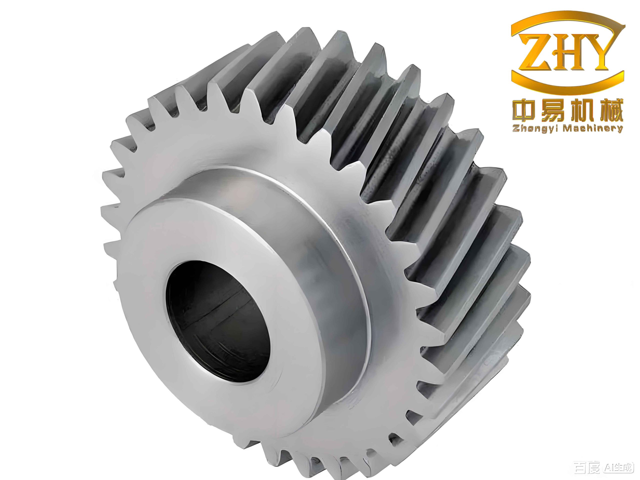
In my work, I designed a dual-camera machine vision system that observes the end face and the side face of helical gears simultaneously. One camera captures the end face for circle parameters and tooth counting. The second camera captures the side face for helix angle and hand-of-helix determination. I then developed image preprocessing, edge extraction, circle fitting, line fitting, and geometric tolerance evaluation algorithms. The final system can measure addendum diameter, dedendum diameter, inner bore diameter, tooth number, helix angle, hand of helix, and concentricity error. The experimental results show that the proposed method is feasible and accurate for helical gears of different specifications.
Overall Measurement Scheme
I treated the helical gear as a part with two main inspection planes. The end face contains concentric circular features: the addendum circle, the dedendum circle, and the inner bore. The side face contains the helical tooth traces, which are the projection of the helical flanks onto the image plane. Because the helix angle is a three-dimensional feature, a single end-face image is not sufficient. Therefore, I used two cameras fixed on a rigid frame. The end-face camera is mounted above the gear, and the side camera is mounted perpendicular to the gear axis. A rotating stage holds the helical gear and allows the side camera to capture the middle tooth region clearly. A stepper-motor-driven lifting mechanism adjusts the working distance of the end-face camera so that helical gears of different sizes remain in focus.
| Subsystem | Design Choice | Function |
|---|---|---|
| End-face camera | 20 MP CMOS, C-mount | Capture addendum, dedendum, inner bore, tooth number |
| Side camera | 20 MP CMOS, C-mount, 12 mm lens | Capture middle tooth edges for helix angle |
| Lighting | High-bright front lighting for end face; low-bright front lighting for side face | Improve edge contrast of helical gears |
| Lifting mechanism | Stepper motor with ball screw slide | Adjust camera working distance for different helical gears |
| Rotating stage | 3D-printed PLA platform driven by a small stepper motor | Align the middle tooth with the side camera |
| Frame | 30 mm x 30 mm aluminum profile | Provide stiffness, modularity, and low weight |
The camera and lens selection followed the required field of view. The largest helical gear in my experiments had a width of about 68 mm, so the minimum field of view was set to 68 mm x 68 mm. The minimum working distance was about 100 mm. I used the standard lens selection relation
$$ f = \frac{WD \cdot H}{FOV} $$
where \(f\) is the focal length, \(WD\) is the working distance, \(H\) is the sensor pixel size, and \(FOV\) is the field of view. Based on this relation, I selected a 12 mm lens with an F2.6 aperture. The camera pixel size was 2.4 µm x 2.4 µm. The image resolution was 5472 x 3648 pixels. This combination provided enough spatial resolution for measuring the main parameters of helical gears with micron-level pixel equivalent.
Camera Calibration and Pixel Equivalent
To convert image pixels into physical dimensions, I calibrated both cameras. The calibration process establishes the relationship between the world coordinate system, the camera coordinate system, the image coordinate system, and the pixel coordinate system. The transformation from world coordinates to camera coordinates is
$$ \begin{bmatrix} X_c \\ Y_c \\ Z_c \\ 1 \end{bmatrix} = \begin{bmatrix} R & t \\ 0 & 1 \end{bmatrix} \begin{bmatrix} X_w \\ Y_w \\ Z_w \\ 1 \end{bmatrix} $$
where \(R\) is the rotation matrix and \(t\) is the translation vector. The pinhole projection from camera coordinates to image coordinates is
$$ Z_c \begin{bmatrix} u \\ v \\ 1 \end{bmatrix} = \begin{bmatrix} f_x & 0 & u_0 & 0 \\ 0 & f_y & v_0 & 0 \\ 0 & 0 & 1 & 0 \end{bmatrix} \begin{bmatrix} R & t \\ 0 & 1 \end{bmatrix} \begin{bmatrix} X_w \\ Y_w \\ Z_w \\ 1 \end{bmatrix} $$
where \(f_x\) and \(f_y\) are the effective focal lengths in pixel units, and \(u_0\) and \(v_0\) are the principal point coordinates. Because real lenses have distortion, I included radial and tangential distortion. The corrected pixel coordinates can be expressed as
$$ x_{dis} = x(1 + k_1 r^2 + k_2 r^4 + k_3 r^6) + 2 p_1 x y + p_2 (r^2 + 2x^2) $$
$$ y_{dis} = y(1 + k_1 r^2 + k_2 r^4 + k_3 r^6) + p_1 (r^2 + 2y^2) + 2 p_2 x y $$
where \(r^2 = x^2 + y^2\), \(k_1\), \(k_2\), and \(k_3\) are radial distortion coefficients, and \(p_1\) and \(p_2\) are tangential distortion coefficients. I used a planar checkerboard with 12 x 9 squares and a square size of 10 mm. The calibration board had a pattern accuracy of 0.01 mm. I captured multiple views for each camera and removed images with large reprojection error. The final calibration parameters are listed in the table below.
| Camera | fx (pixel) | fy (pixel) | u0 (pixel) | v0 (pixel) | k1 | k2 |
|---|---|---|---|---|---|---|
| End-face camera | 5239.91 | 5240.51 | 2712.54 | 1807.74 | -0.08607 | 0.06464 |
| Side camera | 5244.52 | 5243.81 | 2695.64 | 1759.58 | -0.07668 | 0.00693 |
After calibration, I determined the pixel equivalent for the end-face camera. The checkerboard plane gave a pixel equivalent of 0.0676 mm/pixel. Because the helical gear was placed on a rotating platform with a height of 108.9 mm, the actual object distance differed from the calibration plane. Using the small-hole imaging relation and the fixed focal length condition, I corrected the pixel equivalent as
$$ K = K’ \frac{w_2}{w_2 – 108.9} $$
where \(K’\) is the pixel equivalent at the calibration plane and \(w_2\) is the object distance at the calibration plane. The final pixel equivalent for the helical gear end face was 0.0682 mm/pixel. This value was used to convert all end-face measurements from pixels to millimeters.
Image Preprocessing of Helical Gears
Raw images of helical gears contain color information, uneven illumination, noise, and background interference. I preprocessed the images before edge extraction. First, I converted each color image to grayscale using the weighted average method:
$$ G(x,y) = 0.3R(x,y) + 0.59G(x,y) + 0.11B(x,y) $$
This conversion preserved the perceived brightness and reduced the data volume. For the end-face images, the illumination was not perfectly uniform. Some regions of the helical gear were darker than others. To improve the visibility of dark details, I applied a gamma transformation:
$$ V_{out} = A V_{in}^{\gamma} $$
where \(V_{in}\) is the normalized input pixel value, \(V_{out}\) is the output value, \(A\) is a constant, and \(\gamma\) is the gamma coefficient. By choosing \(\gamma\) appropriately, I enhanced the dark regions of the helical gear end face without overexposing the bright regions.
I then compared four denoising filters: Gaussian filtering, median filtering, mean filtering, and bilateral filtering. Gaussian filtering is a linear smoothing operation. Its kernel is based on the Gaussian function:
$$ G(x,y) = \frac{1}{2\pi\sigma^2} e^{-\frac{x^2+y^2}{2\sigma^2}} $$
Median filtering replaces each pixel with the median value in its neighborhood. Mean filtering replaces each pixel with the average value in its neighborhood. Bilateral filtering combines spatial distance and intensity similarity. The comparison is summarized below.
| Filter | Noise Removal | Edge Preservation | Use in My Method |
|---|---|---|---|
| Gaussian | Good for Gaussian noise | Moderate; can blur edges | Used inside LOG edge detection |
| Median | Good for salt-and-pepper noise | Good | Selected for side-face images |
| Mean | Simple and fast | Weak; blurs edges | Not selected |
| Bilateral | Good for smoothing | Strong edge preservation | Not selected due to higher cost |
For the end-face images, I applied Gaussian filtering as part of the LOG edge detection. For the side-face images, I selected median filtering because it removed noise while preserving the helical tooth edges. After denoising, I used Otsu thresholding to segment the helical gear from the background. Otsu thresholding automatically determines a threshold by maximizing the between-class variance. This was more robust than a fixed threshold because the illumination changed slightly between images.
I also used morphological operations to clean the binary images. Corrosion removes small noise points, dilation fills small gaps, opening removes isolated objects, and closing fills small holes. For the end-face binary image, I applied filling to remove internal holes caused by the keyway and surface reflections. I then extracted the outer contour of the helical gear. For the side-face image, I selected a region of interest around the middle tooth and applied morphological processing to obtain a clean tooth profile.
Edge Extraction of Helical Gear Images
Edge detection is critical because all subsequent measurements of helical gears depend on the accuracy of the extracted contour. I studied several traditional edge detectors: Sobel, Laplacian, LOG, and Canny. The Sobel operator uses first-order derivatives. Its horizontal and vertical kernels are
$$ G_x = \begin{bmatrix} -1 & 0 & 1 \\ -2 & 0 & 2 \\ -1 & 0 & 1 \end{bmatrix}, \quad G_y = \begin{bmatrix} -1 & -2 & -1 \\ 0 & 0 & 0 \\ 1 & 2 & 1 \end{bmatrix} $$
The Laplacian operator is a second-order derivative operator. Its common discrete kernel is
$$ \nabla^2 = \begin{bmatrix} 0 & 1 & 0 \\ 1 & -4 & 1 \\ 0 & 1 & 0 \end{bmatrix} $$
Because the Laplacian is sensitive to noise, I combined it with Gaussian smoothing to form the LOG detector. The LOG operator is
$$ \nabla^2 G(x,y) = \frac{\partial^2 G}{\partial x^2} + \frac{\partial^2 G}{\partial y^2} $$
The Canny detector uses Gaussian smoothing, gradient calculation, non-maximum suppression, double thresholding, and edge linking. It is robust for connected edges but can be affected by illumination if the threshold is not selected carefully.
| Algorithm | Behavior on End Face | Behavior on Side Face | Decision |
|---|---|---|---|
| Sobel | Incomplete outer contour | Missing edge segments | Not selected |
| Laplacian | Noise sensitive; some false edges | Weak connection | Not selected alone |
| LOG | Clear and complete contour | Good but less connected | Selected for end face |
| Canny | Good but threshold sensitive | Strong connectivity and smooth edges | Selected for side face |
For the end-face image, I used a combination of gamma transformation and the LOG detector. The gamma transformation improved the dark regions, and the LOG detector extracted a complete contour of the addendum circle, dedendum circle, and inner bore. For the side-face image, I first extracted the region of interest around the middle tooth. I then applied median filtering, Otsu thresholding, and Canny edge detection. This produced two clear helical edge lines for subsequent line fitting.
End-Face Parameter Measurement of Helical Gears
The end-face parameters include the addendum circle diameter, dedendum circle diameter, inner bore diameter, and tooth number. I first located the gear center. The initial center was estimated using the centroid of the contour points:
$$ x_0 = \frac{\sum_{i=1}^{n} x_i}{n}, \quad y_0 = \frac{\sum_{i=1}^{n} y_i}{n} $$
This centroid provided a reference for separating the addendum, dedendum, and inner bore contours. To measure the addendum and dedendum circles, I compared two methods: minimum enclosing circle and least-squares circle fitting. The minimum enclosing circle method finds the smallest circle that contains all addendum points. The maximum inscribed circle method finds the largest circle inside the dedendum contour. These methods are intuitive but sensitive to outliers. The least-squares circle fitting method minimizes the algebraic distance from the points to the circle. The circle equation is
$$ (x – A)^2 + (y – B)^2 = R^2 $$
which can be expanded as
$$ x^2 + y^2 + a x + b y + c = 0 $$
For each contour point \((x_i, y_i)\), the residual is
$$ \delta_i = x_i^2 + y_i^2 + a x_i + b y_i + c $$
I minimized the sum of squared residuals to obtain \(a\), \(b\), and \(c\). The center and radius are then
$$ A = -\frac{a}{2}, \quad B = -\frac{b}{2}, \quad R = \sqrt{A^2 + B^2 – c} $$
I applied this method to the addendum contour, the dedendum contour, and the inner bore contour. The inner bore had a keyway, so I used morphological processing to remove the keyway region before fitting. The comparison between the minimum enclosing circle and least-squares fitting showed that least-squares fitting had smaller error. The addendum error was reduced to 0.29 pixels, while the minimum enclosing circle error was 0.76 pixels. Therefore, I selected least-squares circle fitting for all circular parameters of helical gears.
To count the teeth of helical gears, I used a mask and connected-component analysis. After binarization and filling, the tooth regions form separate connected components. The number of connected components equals the number of teeth. This method is fast and robust to small surface defects. It does not rely on the intersection between the pitch circle and the tooth profile, so it avoids errors caused by local wear or lighting variation. The tooth number is an integer parameter and is essential for calculating the module and the helix angle.
Once the addendum diameter \(d_a\), dedendum diameter \(d_f\), and tooth number \(z\) are known, I calculated the normal module \(m_n\). For standard helical gears, the addendum and dedendum diameters are
$$ d_a = \frac{m_n z}{\cos\beta} + 2 h_a^* m_n $$
$$ d_f = \frac{m_n z}{\cos\beta} – 2(h_a^* + c^*) m_n $$
where \(h_a^*\) is the addendum coefficient and \(c^*\) is the clearance coefficient. According to the standard, \(h_a^* = 1\) and \(c^* = 0.25\). Subtracting the two equations gives
$$ d_a – d_f = 2(2h_a^* + c^*) m_n $$
Thus,
$$ m_n = \frac{d_a – d_f}{2(2h_a^* + c^*)} = \frac{d_a – d_f}{4.5} $$
This normal module is used later in the helix angle calculation. The inner bore diameter is also measured by least-squares fitting. The center of the inner bore and the center of the addendum circle are used for concentricity evaluation.
Side-Face Parameter Measurement of Helical Gears
The helix angle is one of the most important parameters of helical gears. It determines the axial overlap, transmission smoothness, and load distribution. The helix angle is defined as the acute angle between the tangent to the helical line on the reference cylinder and the axis of the helical gear. If the reference cylinder is unwrapped, the helical line becomes a straight line. The relationship between the helix angle, the reference diameter, and the lead is
$$ \tan\beta = \frac{\pi d}{T} $$
where \(\beta\) is the reference helix angle, \(d\) is the reference diameter, and \(T\) is the lead. Similarly, for the addendum circle,
$$ \tan\beta_a = \frac{\pi d_a}{T} $$
Because the lead is constant for a given helical gear, the reference helix angle can be obtained from the addendum helix angle:
$$ \tan\beta = \frac{d}{d_a} \tan\beta_a $$
The reference diameter is
$$ d = \frac{m_n z}{\cos\beta} $$
Substituting this into the previous relation gives
$$ \sin\beta = \frac{m_n z}{d_a} \tan\beta_a $$
Therefore,
$$ \beta = \arcsin\left(\frac{m_n z}{d_a} \tan\beta_a\right) $$
This formula allows me to calculate the helix angle of helical gears from the measured addendum helix angle, the normal module, the tooth number, and the addendum diameter. In practice, the side camera may not be perfectly perpendicular to the gear axis. This alignment error introduces a small offset angle. I corrected this by extracting the edge of the gear boss and fitting a straight line to it. The slope of this line gives the offset angle. I then compensated the addendum helix angle by subtracting the offset angle.
To measure the addendum helix angle, I extracted the region of interest containing the middle tooth. I detected the two edge lines of the middle tooth using Canny edge detection. I then fitted a straight line to each edge:
$$ y = k x + b $$
The slope \(k\) gives the inclination of the tooth edge. The angle of the line is
$$ \theta = \arctan(k) $$
I averaged the angles of the two edges to obtain the measured addendum helix angle. The sign of the slope also determines the hand of helix. If the slope is positive, the helical gear is right-hand. If the slope is negative, the helical gear is left-hand. This classification was correct for all tested helical gears.
Concentricity Measurement of Helical Gears
Concentricity is a geometric tolerance that describes the deviation between the addendum circle center and the inner bore center. For helical gears, poor concentricity causes vibration, noise, and uneven load distribution. I defined the concentricity error as the Euclidean distance between the two fitted centers:
$$ e = \sqrt{(x_1 – x_2)^2 + (y_1 – y_2)^2} $$
where \((x_1, y_1)\) is the addendum circle center and \((x_2, y_2)\) is the inner bore center. Alternatively, the concentricity error can be expressed as the difference between the maximum and minimum radial distances between the addendum contour and the inner bore contour:
$$ e = \max_i (R_i – r_i) – \min_i (R_i – r_i) $$
I used both definitions for cross-checking. The first definition is simpler and directly uses the fitted circle centers. The second definition is more robust when local contour defects exist. In my experiments, the two definitions gave consistent results. The concentricity errors of the tested helical gears were all within 0.1 mm.
Experimental Setup and Measurement Procedure
I built the experimental setup with a rigid aluminum profile frame. The end-face camera was mounted on a stepper-motor-driven lifting slide. The side camera was fixed on the side of the frame. The helical gear was placed on a rotating stage. Two LED bar lights provided front illumination. The end-face light was set to high brightness to create a strong contrast between the helical gear and the background. The side light was set to lower brightness to avoid overexposure on the tooth edges.
The measurement procedure I followed was:
| Step | Operation | Purpose |
|---|---|---|
| 1 | Calibrate both cameras with a planar checkerboard | Obtain intrinsic and extrinsic parameters |
| 2 | Capture end-face and side-face images of helical gears | Acquire raw data |
| 3 | Correct distortion and convert grayscale | Remove lens distortion and reduce data |
| 4 | Enhance end-face image with gamma transformation | Improve dark region visibility |
| 5 | Denoise side-face image with median filtering | Preserve tooth edges |
| 6 | Segment with Otsu thresholding and morphology | Separate helical gears from background |
| 7 | Extract end-face contour with LOG | Obtain addendum, dedendum, and inner bore edges |
| 8 | Extract side-face middle tooth edges with Canny | Obtain helical edge lines |
| 9 | Fit circles and lines | Calculate parameters and hand of helix |
| 10 | Compute module, helix angle, and concentricity | Complete inspection |
Measurement Results for Helical Gears
I tested three helical gears with different modules, tooth numbers, helix angles, and hands of helix. The specifications are listed below.
| Helical Gear | Module (mm) | Tooth Number | Helix Angle (deg) | Hand of Helix |
|---|---|---|---|---|
| 1 | 2 | 30 | 16.8 | Left |
| 2 | 1.5 | 26 | 45.0 | Left |
| 3 | 1.25 | 25 | 19.6 | Right |
The addendum circle measurement results are shown in the next table. The average absolute error was 13.2 µm, and the average relative error was 0.023 percent. The smallest absolute error occurred for the smallest helical gear, which indicates that the pixel equivalent and edge extraction were well controlled.
| Helical Gear | Actual Addendum (mm) | Measured Addendum (mm) | Absolute Error (mm) | Relative Error (%) |
|---|---|---|---|---|
| 1 | 67.40 | 67.3800 | 0.0200 | 0.030 |
| 2 | 57.15 | 57.1358 | 0.0142 | 0.025 |
| 3 | 35.17 | 35.1647 | 0.0053 | 0.015 |
The dedendum circle measurement results are shown below. The average absolute error was 15.4 µm, and the average relative error was 0.035 percent. The dedendum contour is slightly more difficult to extract because the tooth roots are narrower and the transition fillets can be affected by lighting.
| Helical Gear | Actual Dedendum (mm) | Measured Dedendum (mm) | Absolute Error (mm) | Relative Error (%) |
|---|---|---|---|---|
| 1 | 58.35 | 58.3357 | 0.0143 | 0.025 |
| 2 | 45.15 | 45.1287 | 0.0213 | 0.047 |
| 3 | 32.67 | 32.6593 | 0.0107 | 0.033 |
The inner bore measurement results are shown in the next table. The average absolute error was 12 µm, and the average relative error was 0.063 percent. The relative error was slightly larger than that of the addendum circle because the inner bore is smaller and the keyway influences the contour. However, the absolute error remained small.
| Helical Gear | Actual Inner Bore (mm) | Measured Inner Bore (mm) | Absolute Error (mm) | Relative Error (%) |
|---|---|---|---|---|
| 1 | 21.85 | 21.8657 | 0.0157 | 0.072 |
| 2 | 17.78 | 17.7911 | 0.0111 | 0.062 |
| 3 | 15.86 | 15.8513 | 0.0087 | 0.055 |
The helix angle measurement results are shown below. The average relative error was 0.32 percent. The absolute error was less than 0.11 degrees for all tested helical gears. The largest absolute error occurred for the 45-degree helical gear, which is expected because the projected tooth edges become shorter and more sensitive to line fitting. Even so, the relative error was still acceptable.
| Helical Gear | Actual Helix Angle (deg) | Measured Helix Angle (deg) | Absolute Error (deg) | Relative Error (%) |
|---|---|---|---|---|
| 1 | 16.8 | 16.7360 | 0.0640 | 0.38 |
| 2 | 45.0 | 45.1087 | 0.1087 | 0.24 |
| 3 | 19.6 | 19.5364 | 0.0683 | 0.35 |
The concentricity measurement results are shown in the next table. I computed the distance between the fitted addendum center and the fitted inner bore center. All values were below 0.1 mm. This confirms that the proposed vision method can evaluate the concentricity of helical gears in a non-contact manner.
| Helical Gear | Addendum Center (mm) | Inner Bore Center (mm) | Concentricity Error (mm) |
|---|---|---|---|
| 1 | (36.8919, 37.3887) | (36.8509, 37.4209) | 0.05 |
| 2 | (35.7638, 36.2606) | (35.7543, 36.1842) | 0.07 |
| 3 | (38.6584, 39.4563) | (38.5947, 39.4075) | 0.08 |
The overall accuracy is summarized below. The average measurement accuracy of the addendum circle, dedendum circle, and inner bore was within 16 µm. The helix angle relative error was within 0.4 percent. The concentricity error was within 0.1 mm. These results confirm that the dual-camera machine vision method is feasible for helical gears.
| Parameter | Average Absolute Error | Average Relative Error | Remarks |
|---|---|---|---|
| Addendum circle | 13.2 µm | 0.023% | Least-squares circle fitting |
| Dedendum circle | 15.4 µm | 0.035% | Least-squares circle fitting |
| Inner bore | 12.0 µm | 0.063% | Keyway removed by morphology |
| Helix angle | Less than 0.11 deg | 0.32% | Offset angle compensated |
| Concentricity | Less than 0.1 mm | Not applicable | Center distance method |
Software System for Helical Gear Measurement
I also developed a graphical measurement system so that the method can be used without manually editing code. The system was designed in a MATLAB environment. It contains two main interfaces: an image preprocessing interface and a helical gear parameter measurement interface. The preprocessing interface allows the user to load an image, crop the region of interest, convert to grayscale, apply gamma transformation, apply filtering, perform binarization, apply morphological operations, and extract contours. The measurement interface reads the extracted contour points and calculates the parameters of helical gears. It displays the addendum diameter, dedendum diameter, inner bore diameter, tooth number, hand of helix, helix angle, and concentricity error.
| Interface | Main Functions | Output |
|---|---|---|
| Image preprocessing | Load, crop, grayscale, gamma transform, filter, binarize, morphology, contour extraction | Clean contour images and point coordinates |
| End-face measurement | Circle fitting, tooth counting, center extraction | Addendum, dedendum, inner bore, tooth number |
| Side-face measurement | Line fitting, slope analysis, offset compensation | Helix angle and hand of helix |
| Concentricity measurement | Center distance calculation | Concentricity error |
In the preprocessing interface, the user can see the original image and the processed image side by side. This makes it easy to verify that the edge contour of the helical gear is complete. In the measurement interface, the user clicks buttons to perform circle fitting, line fitting, and tolerance calculation. The results are displayed numerically. The system was tested with a 2 mm module, 30-tooth, 16.8-degree left-hand helical gear. The measured addendum diameter was 67.3800 mm, the dedendum diameter was 58.3357 mm, the inner bore diameter was 21.8657 mm, the tooth number was 30, the hand of helix was left, the helix angle was 16.7360 degrees, and the concentricity error was 0.05 mm. These values agree with the manual measurement results and with the theoretical values of the helical gear.
Discussion
The proposed method has several advantages for helical gears. First, it is non-contact, so it does not scratch or deform the tooth surface. Second, it can measure both end-face and side-face parameters in one setup. Third, the dual-camera arrangement reduces the need to rotate the helical gear between measurements. Fourth, the use of least-squares circle fitting and line fitting provides sub-pixel level stability when the contour points are well extracted. Fifth, the offset angle compensation improves the helix angle measurement when the side camera is not perfectly aligned with the gear axis.
There are also limitations. The accuracy of the method depends on the quality of the edge contour. If the tooth surface has oil, scratches, or strong reflections, the edge may be locally distorted. The side-face measurement is sensitive to the length of the visible tooth edge. For large helix angles, the projected edge is shorter, so the line fitting uncertainty increases. The inner bore with a keyway requires morphological processing, and the keyway can influence the fitted center if it is not removed properly. The current system uses a fixed pixel equivalent for the end-face plane. If the helical gear height changes significantly, the working distance and pixel equivalent should be recalibrated or compensated.
For future work, I would improve the system in several ways. I would design a more precise fixture to align the gear axis with the camera optical axis. I would study sub-pixel edge detection algorithms to further improve the contour accuracy. I would apply illumination equalization to reduce the influence of surface reflections. I would also test more helical gears with different modules, pressure angles, and helix angles to build a larger statistical dataset. Finally, I would integrate the measurement system with a production line conveyor and a database so that each helical gear can be traced and classified automatically.
Conclusion
I developed a machine vision method for non-contact parameter detection of helical gears. The method uses two cameras to capture the end face and side face of helical gears. The end-face camera measures the addendum circle, dedendum circle, inner bore, and tooth number. The side camera measures the helix angle and hand of helix. I used gamma transformation and LOG edge detection for the end face, and median filtering plus Canny edge detection for the side face. I used least-squares circle fitting for circular parameters, line fitting for helix angle, and center distance for concentricity. The experimental results show that the average measurement accuracy of the circular parameters is within 16 µm, the helix angle relative error is within 0.4 percent, and the concentricity error is within 0.1 mm. The method is feasible, efficient, and suitable for online inspection of helical gears.
The main contributions of my work can be summarized as follows. I designed a dual-camera image acquisition system for helical gears. I proposed an edge extraction strategy that combines gamma transformation with LOG for the end face and Canny for the side face. I developed a helix angle measurement method that includes offset angle compensation. I implemented a concentricity evaluation method based on the addendum and inner bore centers. I also developed a graphical measurement system that makes the procedure practical for industrial use. The results confirm that machine vision can provide a reliable non-contact alternative for inspecting helical gears with complex tooth geometry.