
In this study, I investigate the meshing characteristics of a hypoid bevel gear pair under different operating conditions. A hypoid bevel gear is a special type of spiral bevel gear whose axes are offset, so the pinion axis does not intersect the gear axis. This offset allows the pinion to have a larger diameter and a larger spiral angle, which improves the strength and rigidity of the pinion. Because of these advantages, hypoid bevel gears are widely used in automotive drive axles, aerospace transmissions, marine propulsion systems, and heavy machinery. However, the geometry of a hypoid bevel gear is complex, and its meshing process involves nonlinear contact, time-varying stiffness, and load-dependent contact patterns. Therefore, accurate modeling and dynamic contact analysis are necessary to evaluate the meshing performance of hypoid bevel gears.
The main objective of my work is to establish a precise finite element model of a hypoid bevel gear pair based on the actual manufacturing process, and then to study the contact stress, contact path, and mesh stiffness under various speeds and loads. I use a Gleason-type generating method for the pinion and a forming method for the gear. The tooth surface equations are derived through coordinate transformations of the cutting machine. Discrete points on the tooth surfaces are calculated numerically and then imported into a three-dimensional modeling environment for surface reconstruction. The assembled model is used for transient dynamic contact analysis. The results provide useful information for tooth surface optimization and manufacturing parameter selection.
Research Background and Significance
Gear transmission is one of the most common mechanical transmission forms. It is used in aviation, aerospace, navigation, energy, transportation, and weapon systems. A gear pair must transmit motion and power smoothly, maintain a stable instantaneous transmission ratio, and possess sufficient load-carrying capacity. A well-designed gear system is compact, space-saving, and has a long service life. The hypoid bevel gear is a spatial gear transmission with intersecting or offset axes. When the offset is zero, the hypoid bevel gear becomes a spiral bevel gear. Therefore, a hypoid bevel gear can be regarded as a special spiral bevel gear. The offset of the pinion axis increases the spiral angle and the pinion diameter, which greatly enhances the pinion strength and stiffness. This increases the spatial freedom and efficiency of the transmission and better meets the requirements of modern machinery.
With the development of science and technology, higher requirements have been put forward for gear speed, life, load capacity, and efficiency. The tooth profile equations, strength calculations, vibration and noise control, friction, temperature, and lubrication theory of hypoid bevel gears have been studied extensively. However, load concentration and reasonable stress distribution on the meshing surface still present difficulties in engineering applications. To analyze the meshing force, stress, and deformation during gear transmission, I establish a finite element model based on a Gleason No. 116 milling machine. The gear is cut by the forming method, and the pinion is cut by the tilt generating method. This model allows me to study the dynamic contact behavior of the hypoid bevel gear under different working conditions.
Research Status of Gear Cutting Machines
The first spiral bevel gear was produced in 1913. In 1919, a machine tool based on a patented invention was developed for spiral bevel gears. In 1923, a machine for hypoid gears was produced using a conical hob and a continuous indexing method. In the 1930s, another company invented a cycloidal-palloid bevel gear and its cutting machine. In 1989, a fully CNC machine tool was developed, which simplified the mechanical structure of traditional machines and improved static and dynamic stiffness and machining accuracy. In the late 1990s, machines for large-size spiral bevel gears were produced. In the early 21st century, CNC milling and grinding machines for large-size spiral bevel gears were developed. In 2003, a new machine design concept was introduced that completely abandoned the traditional generating gear concept.
In my country, the production of spiral bevel gears was initially low. In the 1950s, gear cutting machines were introduced and modified. In the 1960s, a vertical semi-automatic spiral bevel gear milling machine was produced. After the 1980s, certain milling machines became the main gear cutting machines. After the 1990s, automation of spiral bevel gear cutting machines became a new research direction, and CNC machines were developed. In 2005, a CNC machine capable of machining a diameter of 1250 mm was successfully produced. After 2006, research focused on the development and production of large-size high-precision CNC machine tools. In this study, I adopt a Gleason No. 116 milling machine because it has a mature processing method and is widely used in mechanical manufacturing.
Research Status of Three-Dimensional Modeling
In the late 17th century, a Danish scientist proposed using an epicycloid as the tooth profile curve, which marked the birth of gear meshing theory. Because of manufacturing and installation difficulties, epicycloid gears were not widely used. Later, involute profiles and the Camus theorem were proposed. The Camus theorem states that the common normal at the contact point of two gear teeth must pass through the pitch point on the line connecting the two centers. This was the first study of the meshing state between two gear tooth surfaces and established the research direction of contact point trajectory.
In 1946, a complete description of the geometry and kinematics of hypoid gears was published. A pitch surface model of hypoid gears was proposed, which simplified the research model. In 1983, researchers analyzed the maximum contact stress of gear tooth surfaces under different load conditions and determined the stress concentration location at the tooth root. In 1985, an analytical model of a pair of contacting teeth was established using an involute profile, considering material and friction. This model was close to the actual gear model and provided a more accurate model for studying the dynamic characteristics of high-speed gears. In 1990, the cutter outer profile equation and the cutter tip fillet equation were derived, and the tooth surface generation principle was described in detail. A tooth surface modification method for reducing vibration and noise was proposed. In 2003, it was pointed out that evaluating spur gears only by bending stress cannot meet practical requirements. Through finite element analysis of non-standard gears, it was found that balanced bending stress can improve gear strength and durability, and optimizing the tooth root fillet reduced the maximum stress by 10% to 30%.
In 2004, a CAD method was used to simulate the machining process of spiral bevel gears. Solid cutters and blank models were used, and Boolean operations were combined to remove unwanted material incrementally. Kinematic relationships were maintained, and a C language program was developed to generate script files for a solid modeling software package. In 2005, software was developed to accurately model hypoid gears. The software could calculate detailed analytical expressions of the tooth surface. The combination of analytical and finite element methods could effectively analyze contact stress changes under different loads. In 2009, the meshing envelope of a conical gear was obtained through actual transmission, and the generatrix of the conical gear on the theoretical gear bearing contact plane was obtained. An involute conical gear with a conical conjugate surface was established. In 2014, it was noted that traditional worm gears are machined by hobbing machines. Because the curvature radius of the tooth surface is complex, it is difficult to establish an accurate 3D model. Therefore, a new mathematical model was established, and software was developed to directly perform CNC machining of worm gears and spiral bevel gears. By adjusting the input parameters according to the tooth profile obtained on the computer, an accurate 3D model was generated.
In China, traditional spiral bevel gear machining was performed by experienced workers through repeated turning and milling for weeks or even months. This was time-consuming, inefficient, and the resulting gear accuracy was not high. In 1979, the expressions of limit tooth line curvature and limit normal vector were proposed. Based on the relative differential principle, the formula for induced normal curvature was derived, which provided a theoretical basis for parameter setting and adjustment in spiral bevel gear machining. In 1987, a local synthesis method was improved. The original method could only control the meshing characteristics near the reference point, and contact defects might occur far from the reference point. Based on the curvature tensor and moving frame method, an analysis method for third-order contact performance was proposed to control the meshing process. In 1999, unified calculation formulas and iterative algorithms for hypoid bevel gears and spiral bevel gears were proposed, which were of great significance for the development of unified spiral bevel gear standards.
In 2000, a design method was proposed that directly sets parameters affecting transmission efficiency, such as contact path and contact ellipse. This method realized the setting of high-order acceleration parameters of spiral bevel gears. In 2003, a modeling method for hypoid bevel gears was studied based on three-coordinate measurement of tooth surface points, followed by mathematical fitting of discrete points to form a new tooth surface. Contact analysis was carried out and verified by experiments. In 2007, NURBS surface approximation was used to realize solid simulation of gear teeth. The feasibility of this method was proved by comparison with experiments. In 2008, a mathematical model was established according to the machining parameters of the theoretical tooth surface, and discrete points were numerically calculated. The data file was imported into Pro/E to establish only the gear model. In 2009, a three-dimensional geometric modeling method was proposed based on virtual machining in CATIA V5, and the real machining process of spiral bevel gears was studied. In 2014, a gear transmission model was established in Euclidean linear space considering machining errors and machine tool errors. The tooth surface machining accuracy was effectively improved by dynamic compensation and correction of machine tool errors, which laid a foundation for establishing an accurate three-dimensional finite element model.
In summary, existing methods for three-dimensional modeling of hypoid bevel gears can be divided into four categories: (1) proposing tooth surface equations and modeling methods without establishing a three-dimensional model; (2) using relevant equipment to scan existing gears to obtain a three-dimensional model, which is costly and has a long optimization cycle; (3) calculating discrete points by numerical analysis without considering the actual machining state, and only establishing the gear model while ignoring the more complex pinion; (4) using professional software provided by a company to obtain a model for analysis, which only provides results and is not conducive to analysis and research. In this study, I establish a three-dimensional model of both the pinion and the gear of a hypoid bevel gear pair based on the actual machining process, summarizing the achievements and shortcomings of existing literature.
Research Status of Gear Dynamic Analysis
In 1765, the curvature relationship between involute tooth profiles was derived, which laid a solid foundation for the systematic development of gear transmission theory. In 1961, the bending stress during gear meshing was first proposed, and the static contact analysis of gears was completed, marking the birth of the TCA method. In 1977, the LTCA method was proposed considering tooth profile deviation, gear deformation, and support system deformation of involute spur gears. The static transmission error and contact path of the gear pair were solved, and the contact ellipse and load distribution within the ellipse at each contact moment were obtained. In 1981, the loaded contact analysis method under loading conditions was established, which determined the relationship between machining parameters and gear geometric parameters. This was of great significance for optimizing gear geometric parameters, tooth surface modification, and improving gear transmission performance. The LTCA analysis method of spiral bevel gears was further studied, and the transmission error and contact path were analyzed. The tooth surface contact area was determined, which pointed out the correct path for numerical simulation and evaluation of the transmission performance of spiral bevel gears under specific loads.
After 1980, a local synthesis method was proposed, which could accurately control the second-order characteristics of the tooth surface. In 1995, a process for three-dimensional mesh stress analysis of spiral bevel gears using finite element method was proposed. The tooth surface coordinate equation was obtained through coordinate transformation, a finite element model was generated, boundary conditions were defined, and the meshing process of a pair of gear teeth was simulated. In 1997, the three-dimensional finite element contact analysis method for spiral bevel gears was improved. Based on the TCA analysis principle, integrated software was developed to directly calculate the static contact stress and the contact stress variation along the meshing line. The comparison verified that the analytical method provided an effective way to improve the efficiency of gear TCA. In 1999, experimental research on the bending stress of spiral bevel gears used in aerospace was carried out. In static contact, the influence of different speeds and loads on the contact bending stress of gears was determined.
In 2002, based on three-dimensional modeling and finite element method, software was developed to obtain the influence of machining errors and assembly errors on contact stress. The contact stress during meshing after tooth profile optimization was obtained and compared with experimental results. A comprehensive calculation method for the contact stress of spiral bevel gears was proposed. The gear meshing and tooth surface contact process were simulated by computer. The error of a local bearing contact result was not obvious, which provided a way to reduce the vibration and noise of gear transmission. In 2004, a face gear three-dimensional model was used in ANSYS for loaded contact analysis. The contact stress and tooth root bending stress of the face gear were obtained. The loaded contact analysis of a gear model with installation errors and a pinion with tooth profile modification was studied. In 2005, a new method for computer simulation of the gear meshing process was designed. The basic algorithm of tooth surface contact analysis was modified to improve the contact analysis accuracy. The change of tooth surface contact stress during instantaneous loading meshing was analyzed considering installation errors and machining errors, and the calculation was verified by experiments. In 2007, based on gear meshing and kinematic analysis, computer code was developed using the relationship between finite element method and analytical method to solve the transmission error and instantaneous contact pressure of gears.
In 2013, the cutting and meshing processes of spiral bevel gears were simulated. Based on the principle of a numerically stable algorithm, the approximate value of the contact position was solved by discretizing the relative flanks at the contact point. The calculation accuracy depended on the mesh density, and sufficient accuracy could be achieved in a short time. The main advantages were the intuitiveness of the calculation process and the adjustability of the calculation results. In the same year, a complete mating process was used to replace fixed boundary conditions and simplified material behavior in a two-dimensional model by combining a 3D contact surface and finite element method. This provided a complete and effective solution to the problem of inaccurate three-dimensional contact analysis of load, deformation, and stress.
In China, mathematicians used analytical methods to obtain the mathematical model of gear meshing theory, which created conditions for thoroughly analyzing hypoid bevel gear transmission technology. The dynamic characteristics of spiral bevel gears were experimentally studied. In 1987, research on noise and vibration in gear transmission was carried out, and an optimization scheme was proposed. In 1992, a loaded contact analysis and calculation method for locally conjugate gear pairs was proposed. The TCA analysis method was developed by introducing equivalent installation adjustment values and the principle of angular displacement coordination. In 1993, the traveling wave resonance of spiral bevel gears was studied by finite element method, and the influence of gear tooth deformation on gear transmission was calculated.
In 1994, an LTCA analysis method for spiral bevel gears under machining errors and load deformation was proposed. Based on the principle of flexible multibody kinematics, the basic motion equations of two tooth surfaces of spiral bevel gears were constructed. The variation law of tooth surface geometric quantities was analyzed after considering contact deformation, bending deformation, bearing deformation, and support structure deformation at the contact position. An active design method for spiral bevel gear LTCA was also studied, in which parameters affecting LTCA analysis could be selected in the initial design stage. In 1998, an LTCA model very similar to actual gear meshing was used for analysis with high accuracy. The compliance coefficient method was used to calculate the meshing deformation of the gear once, and the change of tooth surface contact stress could be obtained, which shortened the calculation time and improved the calculation efficiency. On this basis, a method for analyzing tooth surface contact and edge contact during hypoid bevel gear meshing was studied.
In 2000, the analysis of spiral bevel gear block fracture caused by transverse vibration of a disc gear was carried out, and it was pointed out that the initial crack was located at the tooth root of the large end. In 2001, combining elastic theory and numerical calculation methods, that is, static contact analysis and dynamic contact analysis, based on the Hertz stress calculation principle of spatial curved surfaces and the traditional tooth surface contact strength calculation formula, the variation law of tooth surface contact stress during gear pair meshing was calculated, and the location of contact stress concentration was pointed out. In 2006, the first 20 modes of a spiral bevel gear system were analyzed using an experimental platform, and the experimental results were compared with finite element calculation results. In 2007, the variation law of gear meshing force was obtained by summarizing contact and collision algorithms. A virtual prototype model was used to simulate an internal meshing gear transmission system under different driving functions, and the simulation results under several conditions were compared and analyzed, which laid a solid foundation for the dynamic analysis of internal meshing gear systems. A dynamic virtual prototype model of a single pair of gears was established. After considering contact friction, the normal meshing force obtained by simulation was consistent with the theoretical value, which proved the correctness of the model. The data obtained could provide a basis for the design and optimization of gear systems. A gear transmission system of a gearbox was taken as the research object. The method of setting boundary conditions was described in detail, and the meshing force of each stage gear was obtained through dynamic simulation.
In 2011, the changes of various parameters during continuous dynamic meshing were studied, and the influence of inertial load on gear meshing characteristics was comprehensively analyzed. In 2014, a finite element method for the misalignment of a bevel gear considering multiple factors was invented. Based on the establishment of an overall three-dimensional finite element model of the main reducer, including gear shafts, bearings, bevel gear transmission system, and reducer housing, the stiffness equation of the gear transmission system and the misalignment of the gear were solved considering thermal expansion, tolerance fit, axial thermal expansion, and housing stiffness. A more realistic comprehensive misalignment of gear transmission was calculated, which laid a foundation for the selection of modification coefficients and the modification of tooth addendum.
In summary, existing literature on contact analysis of hypoid bevel gears mainly includes: (1) TCA analysis obtains the contact strength and bending stress of gear teeth, but cannot obtain the actual change process of deformation, stress, and contact path during meshing; (2) the reducer is analyzed as a whole finite element to obtain transmission efficiency, but the influence of accurate tooth surface precision on gear transmission cannot be obtained, and it cannot guide the determination of parameters in the gear machining process; (3) contact analysis under different working conditions, but most researchers use the same type of working conditions to analyze various dynamic indicators. The influence of load, speed, and friction on each indicator is different, so appropriate working conditions should be selected for analysis according to different objects. In this study, I address the shortcomings in existing gear contact analysis. According to different research objects, I set different speeds to analyze contact stress, different loads to analyze contact path, and the influence of load on mesh stiffness within one cycle.
Research Approach and Main Content
Gleason-type intersecting-axis and offset-axis gear transmissions account for a large share of mechanical transmission in my country. Because of the complex geometric characteristics and meshing process of hypoid bevel gears, the basic problems involved in their transmission generally include the following aspects: selection of gear transmission type, selection of machining machine tool, determination of machining method, setting of machining machine parameters, selection of machining cutters, machine tool errors and assembly errors, determination of gear module and number of teeth, determination of geometric dimensions, selection of gear materials and strength design, analysis of transmission accuracy and calculation of errors, calculation of transmission torque, and calculation of other dimensions related to assembly. At present, the main methods of tooth surface machining are cutter cutting and grinding wheel grinding. The latter generally has low finishing efficiency, while the former has high tooth surface machining accuracy and efficiency, so it is widely used. According to the tooth surface machining principle, it can be divided into two categories: forming method and generating method. In generating method machining, the same cutter is used to machine all required gears, and continuous machining is realized, which greatly improves production efficiency and has been widely used.
Therefore, I use the tilt generating method to machine the pinion of the hypoid bevel gear pair and the forming method to machine the gear. I study the meshing process of the hypoid bevel gear and determine the meshing characteristics from the dynamic aspect. The main purpose is to analyze the changes in tooth surface meshing force, contact stress, and mesh stiffness during meshing under different working conditions and to study the influence of load and speed on gear transmission, so as to guide gear design. The analysis flow is as follows: first, I establish tooth surface equations based on the actual machining machine tool; second, I solve the equations numerically and collect discrete points; third, I reconstruct the tooth surface in three-dimensional software to generate the hypoid bevel gear; fourth, I analyze the contact stress and contact force under different speeds and loads; fifth, I analyze the contact path and mesh stiffness under different loads; finally, I summarize the results and provide an outlook.
Three-Dimensional Modeling of Hypoid Bevel Gears
The meshing principle of gears can be divided into planar meshing and spatial meshing. Planar meshing is used to transmit motion between parallel axes. Spatial meshing is used to transmit motion between parallel, intersecting, and offset axes. The meshing of hypoid bevel gears is a contact motion of two conjugate surfaces with offset axes based on the meshing principle of spiral bevel gears. Using the differential expression of the meshing equation, the normal vector and curvature radius at the reference point can be calculated through the instantaneous meshing relationship of two completely conjugate surfaces. The expressions are:
$$ \mathbf{R}_2 = \mathbf{R}_1 + \mathbf{m} $$
$$ \mathbf{n}_1 = \mathbf{n}_2 $$
where \(\mathbf{R}_1\) is the radius vector of point \(M\) on surface \(S_1\), \(\mathbf{n}_1\) is the unit normal vector at that point, \(\mathbf{R}_2\) is the radius vector of point \(M\) on surface \(S_2\), and \(\mathbf{n}_2\) is the unit normal vector at that point. The meshing process is a relay transmission process of pairs of teeth. The basic law of tooth profile meshing can only ensure a stable transmission ratio during the meshing process of one pair of teeth. Only when the next pair of teeth enters meshing and the previous pair has not completely separated can the gear system transmission be stable throughout the entire meshing process. Therefore, the condition that the speeds of the two meshing tooth surfaces along the normal direction are equal is the analytical expression of the differential model for continuous transmission. The meshing equation should be satisfied:
$$ \mathbf{n} \cdot \mathbf{V}_{12} = 0 $$
Line contact surfaces (completely conjugate surfaces) and point contact surfaces (incompletely conjugate surfaces) both satisfy the basic equations and the meshing equation at the meshing position. This is the theoretical basis for determining gear geometric parameters, and it is also the theoretical basis for gear machining and an effective way to obtain the milling and grinding adjustment parameters of cutters and machine tools.
The key to gear machining is tooth surface machining. Forming method machining uses a cutter to cut the tooth surface in one pass, which greatly improves cutting efficiency. Generating method machining produces involute gears. Considering the machining processes of both the pinion and the gear, it greatly facilitates the design and manufacture of spiral bevel gears, reduces the probability of abnormal meshing during use, and improves production efficiency. Because the meshing of spiral bevel gears is localized conjugate and the tooth profiles of the pinion and gear are asymmetric, the machining principles and methods of the pinion and gear of a spiral bevel gear pair are different. In vehicles such as automobiles and tractors, most spiral bevel gears use the Gleason system. In batch production, the fixed installation method is often used for the gear cutting process. The two tooth surfaces of the gear are used as the reference, and the machining parameters of the two tooth surfaces of the pinion are adjusted to obtain a good meshing contact area and backlash.
The machining of spiral bevel gears is realized by assuming a flat-top gear that rotates concentrically with the machine cradle and meshes completely conjugately with the gear being cut. This imaginary gear is called the generating gear. When the blank and the generating gear rotate around their respective axes, the cutter will cut a tooth slot on the blank. The cutting process is consistent with the meshing process of a hypoid bevel gear. To achieve continuous cutting, the rotation direction of the head milling cutter and the gear blank is opposite. When the next milling head begins to cut the tooth slot, the previous milling head has completed the current cutting, and the blank rotates to the next tooth slot position. This process is repeated until all tooth slots are cut.
In theory, the pitch cone of a hypoid bevel gear is an approximation of a single-leaf hyperboloid, and the pitch surfaces during transmission are a pair of hyperboloid surfaces of revolution. However, in practical production and application, because hypoid bevel gears are difficult to machine and the structure is not compact when the transmission ratio is large, a pair of conical surfaces tangent at one point is used as the pitch surfaces, called the indexing cones. The tangent point of the two indexing cones is point \(M\), and its position determines the transmission characteristics of the gear. The included angle between the gear axes is \(\Sigma\), the offset distance between the gear axes is \(E\), the pitch circle radius of the gear is \(r_2\), the pitch circle radius of the pinion is \(r_1\), the offset angle of the gear in the axial section is \(\varepsilon_2\), the offset angle of the pinion in the axial section is \(\varepsilon_1\), and the offset angle of the gear pair is \(\varepsilon\). In the plane \(H_1H_2M\), points \(H_1\) and \(H_2\) are the cone apices of the pinion and gear, respectively. The line \(K_1K_2\) is the pitch perpendicular. \(R_1\) and \(R_2\) are the cone distances of the gears. \(\eta_1\) and \(\eta_2\) are the pitch cone angles of the pinion and gear, respectively.
For a given transmission ratio, the pitch cones of a hypoid bevel gear are not unique. If the spiral angle of the pinion is given, the pitch cones of the hypoid bevel gear are uniquely determined. Therefore, if the spiral angle does not meet the requirements, it can be satisfied by changing the pinion radius \(r_1\). The transmission of a hypoid bevel gear pair is related to the spiral angle, and the spiral angle is determined by the position of the node \(M\) and the speed ratio. The relationship can be expressed as:
$$ \frac{r_1}{r_2} = \frac{z_1}{z_2} = \frac{R_1 \cos \beta_1}{R_2 \cos \beta_2} = \frac{\sin \delta_2}{\sin \delta_1} $$
The limit pressure angle of the gear usually relates to the limit condition of tooth meshing. At this time, the curvature radius of the tooth profile at the instantaneous center of relative motion is zero, and the meshing line shrinks to a point. To obtain the same meshing conditions on both sides of the gear teeth, the difference between the pressure angles on both sides and the limit pressure angle should be equal:
$$ \tan \alpha^* = \frac{R_1 \sin \beta_1 – R_2 \sin \beta_2}{R_1 \tan \delta_1 – R_2 \tan \delta_2} $$
Establishment of Pinion Tooth Surface Equation
Because the structure of the hypoid bevel pinion is relatively complex, I use the tilt generating method to machine the pinion. The tooth slot is machined during the process in which the blank and the generating gear rotate around their respective axes at a stable transmission ratio. This method is called the generating method. It uses the forced meshing motion relationship between the gear cutter and the tooth blank to cut the gear tooth profile.
I establish several coordinate systems for the machine tool. The fixed coordinate system of the machine tool is \(\{O_j, X_j, Y_j, Z_j\}\). The cradle coordinate system is \(\{O_t, X_t, Y_t, Z_t\}\). The base coordinate system of the pinion blank is \(\{O_{bj}, X_{bj}, Y_{bj}, Z_{bj}\}\). The guide rail motion coordinate system is \(\{O_b, X_b, Y_b, Z_b\}\). The pinion blank motion coordinate system is \(\{O_L, X_L, Y_L, Z_L\}\). The pinion blank fixed coordinate system is \(\{O_{Lj}, X_{Lj}, Y_{Lj}, Z_{Lj}\}\). When machining the pinion, the machine tool parameters include the total cutter tilt angle \(\beta\), the total cutter rotation angle \(\eta\), the deflection angle \(\xi\), the angular cutter position \(\theta\), the pinion blank installation angle \(\alpha\), the vertical wheel position \(H_1\), the offset distance \(E_1\), the bed position \(a_1\), and the horizontal wheel position \(b_1\).
The transformation matrix from the fixed coordinate system to the pinion blank fixed coordinate system is:
$$ M_L = \begin{bmatrix}
1 & 0 & 0 & b_1 \\
0 & \cos\gamma & -\sin\gamma & 0 \\
0 & \sin\gamma & \cos\gamma & 0 \\
0 & 0 & 0 & 1
\end{bmatrix} $$
The transformation matrix from the pinion blank fixed coordinate system to the guide rail motion coordinate system is:
$$ M_Y = \begin{bmatrix}
\cos\alpha & -\sin\alpha\cos\theta & \sin\alpha\sin\theta & -H_1 \\
\sin\alpha & \cos\alpha\cos\theta & -\cos\alpha\sin\theta & -a_1 \\
0 & \sin\theta & \cos\theta & 0 \\
0 & 0 & 0 & 1
\end{bmatrix} $$
The transformation matrix from the guide rail motion coordinate system to the cutter coordinate system is:
$$ M_D = \begin{bmatrix}
1 & 0 & 0 & E_1 \\
0 & \cos\xi & -\sin\xi & 0 \\
0 & \sin\xi & \cos\xi & 0 \\
0 & 0 & 0 & 1
\end{bmatrix}
\begin{bmatrix}
\cos\eta & -\sin\eta & 0 & 0 \\
\sin\eta & \cos\eta & 0 & 0 \\
0 & 0 & 1 & 0 \\
0 & 0 & 0 & 1
\end{bmatrix}
\begin{bmatrix}
\cos\beta & 0 & \sin\beta & 0 \\
0 & 1 & 0 & 0 \\
-\sin\beta & 0 & \cos\beta & 0 \\
0 & 0 & 0 & 1
\end{bmatrix} $$
where \(\theta = \omega_1 t\), \(\omega_1\) is the cradle angular velocity, \(\gamma = i \omega_1 t\), and \(i\) is the roll ratio between the generating gear and the workpiece. According to the matrix transformation relationships between the auxiliary coordinate systems, the position vector \(\mathbf{r}\) of the cutting point \(M\) on the cutter in the blank motion coordinate system is derived, which is the pinion tooth surface equation:
$$ \mathbf{R}_L = M_D M_Y M_L \mathbf{r} $$
The pinion of a hypoid bevel gear pair can be machined by either a planar generating gear or a conical generating gear. When the degree of freedom of the generating gear needs to be increased, a planar generating gear should be selected so that the transmission ratio between the generating gear and the blank is variable. When a constant transmission ratio needs to be output, a conical generating gear should be selected to make the transmission system stable. I choose a Gleason No. 116 milling machine with a cutter tilt and cutter rotation cradle mechanism to machine the gear.
Let \(M\) be an arbitrary point on the cutting surface. \(r_c\) is the cutter tip radius. \(S_p\) is the distance from the cutter tip to \(M\). \(\mu\) is the cutter profile angle when cutting the pinion. \(\varepsilon\) is the phase angle of point \(M\). The position vector and normal vector of point \(M\) in the cutter coordinate system \(\{O_d, X_d, Y_d, Z_d\}\) for cutting the pinion are:
$$ \mathbf{r} = \begin{bmatrix}
(r_c + S_p \sin\mu) \cos\varepsilon \\
(r_c + S_p \sin\mu) \sin\varepsilon \\
-S_p \cos\mu \\
1
\end{bmatrix} $$
$$ \mathbf{n} = \begin{bmatrix}
\cos\mu \cos\varepsilon \\
\cos\mu \sin\varepsilon \\
-\sin\mu \\
1
\end{bmatrix} $$
According to the meshing principle, the tooth surface of the generating gear and the tooth surface of the gear tooth satisfy the basic equations and the meshing equation. Let \(\mathbf{v}_{12}\) be the relative motion velocity between the cutter coordinate system and the blank motion coordinate system. \(\omega_1\) is the angular velocity of the cutter coordinate system, and \(\omega_2\) is the angular velocity of the blank motion coordinate system. \(\omega_{12}\) is the relative angular velocity of the two coordinate systems. \(m\) is the center distance between the two coordinate systems. The system of equations should be satisfied:
$$ \begin{cases}
\mathbf{v}_{12} = \mathbf{v}_1 – \mathbf{v}_2 = \omega_1 \times \mathbf{r}_1 – \omega_2 \times \mathbf{r}_2 \\
\mathbf{n} \cdot \mathbf{v}_{12} = 0 \\
\mathbf{r}_1 = M_{1j} \mathbf{r} \\
\mathbf{r}_2 = M_{2j} \mathbf{r} \\
\omega_{12} = \omega_1 – \omega_2 \\
\mathbf{v}_{12} = \omega_{12} \times \mathbf{r} – \mathbf{v}_m
\end{cases} $$
Combining the above equations and simplifying, the pinion tooth profile equation is:
$$ \mathbf{R}_1 = G(\varepsilon, t) $$
Establishment of Gear Tooth Surface Equation
I use the forming method to machine the gear. During the machining process, the machine cradle is fixed. The coordinate systems for gear machining are: the fixed coordinate system of the machine tool \(\{O_{j2}, X_{j2}, Y_{j2}, Z_{j2}\}\), the gear blank fixed coordinate system \(\{O_{Lj2}, X_{Lj2}, Y_{Lj2}, Z_{Lj2}\}\), and the gear blank motion coordinate system \(\{O_{L2}, X_{L2}, Y_{L2}, Z_{L2}\}\). \(a_2\) is the bed position, \(b_2\) is the horizontal wheel position, \(H_2\) is the vertical wheel position, \(\alpha_2\) is the blank installation angle, and \(\gamma_2\) is the rotation angle of the blank around its axis.
The transformation matrices are:
$$ M_{L2} = \begin{bmatrix}
\cos\gamma_2 & -\sin\gamma_2 & 0 & 0 \\
\sin\gamma_2 & \cos\gamma_2 & 0 & 0 \\
0 & 0 & 1 & E_2 \\
0 & 0 & 0 & 1
\end{bmatrix} $$
$$ M_{Y2} = \begin{bmatrix}
\cos\alpha_2 & 0 & \sin\alpha_2 & b_2 \\
0 & 1 & 0 & 0 \\
-\sin\alpha_2 & 0 & \cos\alpha_2 & 0 \\
0 & 0 & 0 & 1
\end{bmatrix} $$
$$ M_{D2} = \begin{bmatrix}
1 & 0 & 0 & 0 \\
0 & 1 & 0 & H_2 \\
0 & 0 & 1 & a_2 \\
0 & 0 & 0 & 1
\end{bmatrix} $$
When the gear is machined by the forming method, the generating gear is a planar generating gear. At this time, the gear tooth surface is exactly the same as the surface of the cutting edge. During the indexing machining of the end milling cutter, each tooth flank is machined as a conical surface. In the cutter coordinate system \(\{O_{d2}, X_{d2}, Y_{d2}, Z_{d2}\}\), \(r_{c2}\) is the cutter tip radius, \(S_{p2}\) is the length from the cutting edge to the cutter tip, \(\mu_2\) is the cutter tilt angle, that is, the pressure angle, and \(\varepsilon_2\) is the phase angle of point \(M\). The position vector and normal vector of point \(M\) in the cutter coordinate system for machining the gear are:
$$ \mathbf{r}_2 = \begin{bmatrix}
(r_{c2} – S_{p2} \sin\mu_2) \cos\varepsilon_2 \\
(r_{c2} – S_{p2} \sin\mu_2) \sin\varepsilon_2 \\
-S_{p2} \cos\mu_2 \\
1
\end{bmatrix} $$
$$ \mathbf{n}_2 = \begin{bmatrix}
\cos\mu_2 \cos\varepsilon_2 \\
\cos\mu_2 \sin\varepsilon_2 \\
-\sin\mu_2 \\
1
\end{bmatrix} $$
Combining the coordinate transformation matrices and the meshing equation, the gear tooth surface equation is:
$$ \mathbf{R}_2 = G_2(\varepsilon_2, t) $$
Three-Dimensional Model Establishment
For a hypoid bevel gear, although the number of teeth can be selected arbitrarily, in general, the number of teeth of the pinion should not be less than 5, and the sum of the teeth of the pinion and gear should not be less than 40. The pitch circle diameter \(d_2\) of the gear is determined in advance according to the load-carrying capacity of the gear. However, there is no general formula or chart available at present. Therefore, I refer to the method for spiral bevel gears and select the pitch circle diameter of the pinion according to empirical formulas or corresponding charts, and then convert it to the pitch circle diameter of the gear according to the transmission ratio. This is used as the initial value of the pitch circle diameter of the hypoid bevel gear. Whether the pitch circle diameter of the gear is appropriate still needs to be checked by strength calculation. If it does not meet the requirements, it should be increased accordingly. After determining the pitch circle diameter, the end face module of the bevel gear at the large end is equal to the pitch circle diameter divided by the number of teeth. Theoretically, increasing the tooth width can increase the strength and life of the gear teeth, but this will also greatly weaken the small end and requires a smaller cutter tip width and tip fillet, which is very unfavorable for manufacturing and reducing tooth root stress concentration. If the load is concentrated at the small end under actual working conditions, the gear teeth will be damaged faster. The gear parameters are listed in Table 1, and the machine tool parameters are listed in Table 2.
| Gear | Number of teeth | Pitch diameter (mm) | Outer diameter (mm) | Pitch cone angle (°) | Face cone angle (°) | Root cone angle (°) | Arc tooth height (mm) | Face width (mm) |
|---|---|---|---|---|---|---|---|---|
| Gear | 30 | 103.02 | 103.91 | 68.44 | 64.98 | 60.66 | 18.80 | 20 |
| Pinion | 14 | 57.49 | 78.27 | 28.47 | 25.02 | 20.70 | 7.55 | 20 |
| Item | Value |
|---|---|
| Pinion root cone angle (°) | -3.18 |
| Pinion horizontal wheel position (mm) | 1.76 |
| Pinion bed position (mm) | 20.51 |
| Pinion vertical wheel position (mm) | 40.73 |
| Cutter eccentric angle (°) | 92.13 |
| Cutter cradle angle (°) | 108.41 |
| Roll ratio | 6.33912 |
| Cutter tip diameter (mm) | 285.52 |
| Cutter profile angle (°) | 20 |
| Cutter tip fillet (°) | 2.59 |
| Gear installation root cone angle (°) | 76.40 |
| Gear horizontal wheel position (mm) | -1.10 |
| Gear horizontal installation distance (mm) | 100.09 |
| Gear vertical installation distance (mm) | 122.43 |
| Gear cutter diameter (mm) | 304.80 |
| Gear profile angle (°) | 22.50 |
| Gear cutter tip fillet radius (°) | 2.29 |
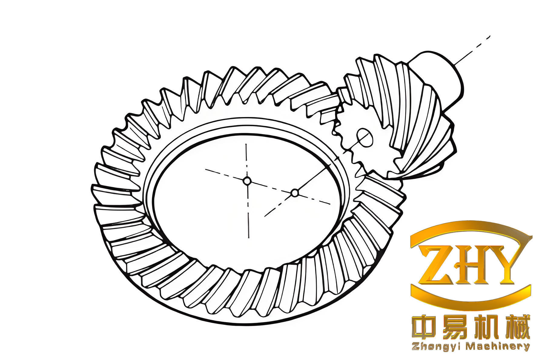
To obtain the tooth surface, I use a numerical calculation method based on the derived tooth surface equations. Combining the basic geometric relationships of the hypoid bevel gear with the gear and machine tool parameters, I write a program to calculate the three-dimensional coordinates of the discrete points on the tooth surface and save them as an ibl file for subsequent surface modeling. The discrete points are imported into Pro/E. In the Pro/E work interface, I select “Insert” → “Datum Curve” and set the reference coordinate system. I call the discrete point set file and follow the order of point, line, surface, and solid to gradually generate the tooth root cone, tooth top cone, and back cone surfaces. Then I trim and adjust the curved tooth surface. After merging and solidifying the obtained surfaces, a single tooth slot is obtained. Through the array function, the other teeth are generated. Finally, I fill and pin the holes to complete the three-dimensional data processing and solid modeling of the hypoid bevel gear. The assembled model of the hypoid bevel gear pair is shown as follows.
Contact Stress Analysis under Different Working Conditions
Gears lose their service effectiveness mainly due to tooth breakage, pitting, and wear during meshing. To extend the service life and improve the strength of gear teeth, contact analysis of gear transmission is necessary. The gear mechanism mainly transmits power through the push of the driving wheel on the driven wheel, realizing the mutual transformation of planar axis and spatial axis gear meshing transmission and changing the output shaft speed. Because gear transmission is relatively precise, it is widely used in high-speed and precise transmission systems. By analyzing the contact stress and contact force of gears, the influence of different actual cutting amounts on gear meshing can be controlled in advance, thereby reducing the time for trial cutting gears. This provides an effective method for significantly improving gear manufacturing processes and quality.
Contact is a very common physical phenomenon and can be used to analyze dynamic impact, friction, metal forming, bolted joints, part assembly, tight assembly, pressure boundary conditions, and sealing devices. The main idea of TCA is based on simulating the contact of two meshing tooth surfaces, determining the instantaneous contact ellipse, and analyzing the meshing and contact of the gear. Based on the principal curvatures and principal directions of the two contacting tooth surfaces, determining the machine tool and cutter installation adjustment values that improve the meshing and contact state is the main subject of gear synthesis. The local contact synthesis of hypoid bevel gears is based on the assumption that the machine tool and cutter installation adjustment values of the gear are already given, and the principal curvatures and principal directions of the gear at the central contact point are also known.
According to the local contact synthesis method, the meshing state of the gear is determined, thereby determining the cutter tilt and cutter rotation structure of the pinion machining machine tool and the installation adjustment values of the machining cutter, which improves the contact state and meshing characteristics within the central contact point \(M\) and its neighborhood. I set up three coordinate systems \(S_{11}\), \(S_{22}\), and \(S_f\) rigidly fixed to gear 1, gear 2, and the frame, respectively, and an additional fixed coordinate system \(S_q\). Assume that a tooth surface family is formed by gear 1 rotating around a fixed axis located in \(S_f\). Therefore, the tooth surface family and unit normal equation are:
$$ \mathbf{r}_1^{(1)} = M_{f1} \mathbf{r}_1 $$
$$ \mathbf{n}_1^{(1)} = L_{f1} \mathbf{n}_1 $$
When establishing the gear meshing model for analysis, parameters are set to compensate for machine tool errors and installation errors, and the vector expression of the coordinate system \(S_q\) in the coordinate system \(S_f\) is expressed. The tooth surface family and unit normal vector equations of gear 2 are:
$$ \mathbf{r}_2^{(2)} = M_{fq} M_{q2} \mathbf{r}_2 $$
$$ \mathbf{n}_2^{(2)} = L_{fq} L_{q2} \mathbf{n}_2 $$
In reality, contacting objects do not penetrate each other. Therefore, the finite element analysis software must coordinate the two contact surfaces to avoid mutual penetration of their finite element models. The process of preventing penetration is called forced contact coordination. In Workbench, there are five different algorithms to achieve contact surface coordination: augmented Lagrange method, pure penalty function method, multi-point constraint method for both tangential and normal directions, pure Lagrange method only in the normal direction with pure penalty function method in the tangential direction, and pure Lagrange method in both normal and tangential directions. In this study, I use the augmented Lagrange method because it provides good convergence for nonlinear contact problems.
Finite element analysis is a method that uses mathematics and mechanics knowledge and computer technology to solve engineering technical problems. Theoretically, an infinite set of simple functions can approximate a complex original function. Using the same principle, a large number of discrete elements are used to replace a complex arbitrary geometric shape. By analyzing the displacement, stress, and strain within the discrete set under external forces, accurate information about the internal mechanics of the geometric body can be obtained. Therefore, in gear contact analysis, a geometric discrete set of several finite-sized elements represents any continuous body. The required mechanical values are obtained by comprehensively solving the deformation of the nodes of any two mutually hinged elements. This provides a good approximate solution for solving partial differential equations. The finite element solution idea can be applied to problems with different physical properties and mathematical models. The difference lies in the derivation formula, solution conditions, and calculation process. The finite element solution idea is generally divided into six steps: determine the problem to be solved and clarify the solution direction; determine the definition of the solution domain and boundary to avoid obtaining meaningless solution sets that affect the analysis results; discretize the problem to be solved with a finite number of elements; determine the variables, the definition domain of the variables, and the method of controlling the variables; derive the equation for each element and establish the element function; solve the system of equations and analyze and verify the results.
Dynamic analysis first requires the establishment of a finite element model. Models are mainly divided into three categories: mechanical components, multi-rigid-body systems, and multi-flexible-body systems. The finite element modeling method for mechanical component dynamics is relatively mature. Commercial software such as ANSYS and NASTRAN can perform dynamic modeling and analysis, but the multi-rigid-body dynamics method and software for mechanical systems with moving parts lag far behind. The technology of multi-rigid-body system dynamics modeling is relatively mature and can be completed on commercial software such as ADAMS. There are deficiencies in the unified modeling of multi-rigid-body systems and electromechanical coupling systems with singularities and redundant degrees of freedom. The basic idea of multi-flexible-body system modeling is to obtain a generalized coordinate basis for the finite-dimensional approximation of flexible body dynamics based on finite element, assumed mode, corrected mode, and singular perturbation methods combined with joint variables. However, it is far from reaching the engineering level of deriving dynamic equations through Lagrange equations or variational principles. Transient dynamics is a method for analyzing the dynamic response of an analysis object to arbitrarily varying loads over time. It obtains the changes in displacement, strain, stress, and force over time under arbitrary load states (steady state, transient state, harmonic). The load-time correlation makes inertial and damping effects relatively important.
$$ [M]\{\ddot{u}\} + [C]\{\dot{u}\} + [K]\{u\} = \{F(t)\} $$
where \([M]\) is the structural global mass matrix, \([C]\) is the structural global damping matrix, \([K]\) is the structural global stiffness matrix, \(\{u\}\) is the structural nodal displacement vector, and \(t\) is the load action time. At any given time \(t\), this equation is converted into a static equilibrium equation, and the loads of inertial force and damping force are taken into account. ANSYS provides two solution methods: the Newmark time integration algorithm and the improved HHT algorithm. The implicit method using finite difference within a time interval is:
$$ \{\dot{u}_{n+1}\} = \{\dot{u}_n\} + [(1-\delta)\{\ddot{u}_n\} + \delta \{\ddot{u}_{n+1}\}] \Delta t $$
$$ \{u_{n+1}\} = \{u_n\} + \{\dot{u}_n\} \Delta t + \left[ \left( \frac{1}{2} – \alpha \right) \{\ddot{u}_n\} + \alpha \{\ddot{u}_{n+1}\} \right] \Delta t^2 $$
The displacement at the next moment \(u_{n+1}\) is combined with the control equation at \(t_{n+1}\):
$$ \{\ddot{u}_{n+1}\} = a_0 (\{u_{n+1}\} – \{u_n\}) – a_2 \{\dot{u}_n\} – a_3 \{\ddot{u}_n\} $$
$$ \{\dot{u}_{n+1}\} = \{\dot{u}_n\} + a_6 \{\ddot{u}_n\} + a_7 \{\ddot{u}_{n+1}\} $$
where \(a_0 = \frac{1}{\alpha \Delta t^2}\), \(a_1 = \frac{\delta}{\alpha \Delta t}\), \(a_2 = \frac{1}{\alpha \Delta t}\), \(a_3 = \frac{1}{2\alpha} – 1\), \(a_4 = \frac{\delta}{\alpha} – 1\), \(a_5 = \frac{\Delta t}{2} \left( \frac{\delta}{\alpha} – 2 \right)\), \(a_6 = \Delta t (1 – \delta)\), and \(a_7 = \delta \Delta t\).
In ANSYS, the steps for solving contact problems are finite element preprocessing (material, model, mesh), setting boundary conditions (contact pairs, rotating pairs, etc.), stress functions (internal stress and external stress functions), and load types (steady, harmonic, transient). When setting the boundary conditions for gear contact analysis, I first set the contact pair. Since the driving wheel is the pinion and the driven wheel is the gear, I set the outer contour surface of the pinion as the target surface and the outer contour surface of the gear as the contact surface. The contact type is frictional contact, and the friction coefficient is 0.1. The gear meshing working conditions are listed in Table 3. I solve the contact stress under six different working conditions.
| Condition | Pinion speed (r/min) | Driven gear load (N·m) |
|---|---|---|
| A | 600 | 0 |
| B | 600 | 50 |
| C | 600 | 200 |
| D | 1200 | 0 |
| E | 1200 | 50 |
| F | 1200 | 200 |
Before initializing the finite element solution, I check whether the analysis data is correct to avoid inaccurate results. When the input model is incomplete or inaccurate, such as insufficient constraints, gaps in the model, or negative material parameters, the force during the finite element calculation process will not converge, and the solution process cannot be completed. Therefore, checking the data before solving is very necessary. It can improve analysis efficiency and avoid useless work. When a suitable integration method is selected for solving, the force results will converge to the exact solution, indicating that the error of the intermediate quantities has little influence on the results and the stability of the mathematical calculation method is good. The meshing of a hypoid bevel gear is nonlinear contact, so I choose the augmented Lagrange function as the analysis function. At the same time, I choose time step control to solve the process, allowing for convergence behavior bisection and time step size adjustment, which provides additional convergence enhancement.
The finite element model is established in ANSYS. I use the geometric model built by the method described above and import it into Hypermesh for meshing. I refine the tetrahedral mesh on the contact tooth surface to obtain a more accurate mesh model, which is then imported into Workbench. The pinion and gear are made of the same material. The elastic modulus is set to \(1.9 \times 10^{11}\) Pa, the Poisson’s ratio is 0.31, and the density is 7800 kg/m\(^3\). The gear contact is set as frictional contact with a friction coefficient of 0.1. The pinion is the driving wheel. In the mesh division detail settings panel, the relevance center is set to “Fine”, and the other settings remain default. The mesh model produces 50,892 nodes and 9,835 elements. The mesh elements are basically hexahedral. The minimum aspect ratio is 1.0498, and the maximum is 3.3736. The usual requirement for this parameter is less than 5, so the aspect ratio quality is high. The maximum warping angle factor is 0.022, and the usual standard warping angle is less than 5°, so the warping angle of this model is very small. The Jacobian ratio is 0.61, and the usual requirement for finite element models is about 0.6. In summary, the mesh quality of this finite element model is relatively high.
The contact stress of gears causes surface damage and contact fatigue under long-term action. Therefore, the maximum contact stress is generally used to measure the service life of gears. Line contact and point contact are distinguished according to the initial geometric conditions of the contact surface. Gear contact is generally line contact, while rolling bearing contact is generally point contact. When designing a hypoid bevel gear, the life should be checked according to the load and size to ensure the safety and reliability of its operation. The contact stress at the meshing point of the gear and the contact stress at the lowest part of the single-tooth meshing area of the pinion should be calculated to reduce the possibility of gear failure and ensure normal gear meshing. The contact ratio of a hypoid bevel gear is relatively large, so the single-tooth meshing contact stress expression is very complex and more difficult to solve. From the modeling in the previous section, the number of teeth of the pinion is 14, so the contact calculation is carried out based on the pitch point meshing. The basic formula for contact stress of a Gleason-type hypoid bevel gear in theoretical design is:
$$ S_c = C_p \left( \frac{T_{Pmx}}{T_P} \right) \left( \frac{C_O C_V C_s C_m C_f}{I F_G D} \right) \left( \frac{N}{n} \right) $$
where \(S_c\) is the maximum contact stress of the tooth surface, \(C_p\) is the elastic coefficient of the gear material, \(T_{Pmx}\) is the maximum transmitted torque of the pinion, \(T_P\) is the transmitted torque of the pinion, \(C_O\) is the overload factor for durability, \(C_V\) is the dynamic factor for durability, \(C_s\) is the size factor for durability, \(C_m\) is the load factor for durability, \(C_f\) is the surface condition factor for durability, \(I\) is the geometry factor for durability, \(F_G\) is the face width of the gear, \(D\) is the outer diameter of the gear, \(N\) is the number of teeth of the gear, and \(n\) is the number of teeth of the pinion. The elastic coefficient is:
$$ C_p = \sqrt{ \frac{3}{2\pi \left( \frac{1-\mu_P^2}{E_P} + \frac{1-\mu_G^2}{E_G} \right)} } $$
where \(\mu_G\) is the Poisson’s ratio of the gear material, \(\mu_P\) is the Poisson’s ratio of the pinion material, \(E_G\) is the elastic modulus of the gear material, and \(E_P\) is the elastic modulus of the pinion material.
From the contact stress analysis, I obtain the von Mises stress distribution during the meshing process under six working conditions. The curves of the maximum von Mises stress versus time are shown in the analysis results. At the beginning, the maximum von Mises stress is relatively small and then gradually increases. At 0.0125 s, the maximum contact von Mises stress of the gear reaches 300 MPa, reaching a high value, and then the gear operates basically smoothly. However, at 0.0375 s, the gear stress suddenly increases and then the gear transmission system tends to be stable again. Observing the curves of the six working conditions, the trend is basically the same. At the beginning, the gear speed increases slowly. During this process, the maximum von Mises stress is relatively small, and the gear transmission is relatively stable without large fluctuations. At a certain moment, when the gear speed reaches the maximum value (the preset speed value), the maximum contact von Mises stress of the gear also reaches the maximum. As the gear continues to transmit, when the gear speed and the applied torque remain unchanged, the gear transmission is basically stable again. After a period of time, due to the change of the gear meshing state, the load distribution changes suddenly, and the meshing stress increases instantaneously, and then the gear transmission system tends to be stable again. The maximum von Mises stress value does not change significantly.
By comparing condition A with condition D, condition B with condition E, and condition C with condition F, I can see that the trend of the contact von Mises stress versus time curve is almost the same under different speeds, but the maximum contact von Mises stress value of the gear increases with the increase of speed. Therefore, speed has a significant influence on the maximum contact stress of the gear. The higher the speed, the greater the maximum contact von Mises stress of the gear. At the same time, the influence of the change of gear meshing state, that is, the change of the number of meshing tooth pairs, on the instantaneous contact stress decreases with the increase of speed. Therefore, gear transmission is more stable at high speed.
By comparing conditions A, B, and C, and conditions D, E, and F, I can see that the trend of the contact von Mises stress versus time curve is almost the same under different loads, but the maximum von Mises stress value of the gear increases with the increase of load. Therefore, load has a certain influence on the maximum contact stress of the gear. The heavier the load, the greater the maximum contact von Mises stress of the gear. By comparing conditions A and B, conditions A and C, conditions D and E, and conditions D and F, it is easy to obtain that under low load conditions, the influence of load on contact is small, and the change of speed has a greater influence on the maximum contact stress.
Contact Path and Mesh Stiffness under Different Loads
The analysis of the contact point path of gear teeth is the basis of dynamic analysis and calculation. The normal contact force of the gear and the deformation along the meshing line are important factors affecting gear meshing vibration and dynamic load. The gear contact pattern can intuitively represent the gear transmission state and gear accuracy. Therefore, based on the finite element principle of spiral bevel gear contact analysis, I establish a suitable coordinate system to obtain the position change data of the meshing point under different working conditions. The discrete points are imported into Matlab for fitting to obtain the meshing point trajectory, and the change of the contact trajectory is analyzed to determine the influence of load on the contact trajectory of the hypoid bevel gear, which lays a foundation for the next step of dynamic characteristics of the gear transmission system.
The tooth surface contact trace is the contact spot distributed on the gear surface under micro-braking. The tooth surface contact spot is the contact area expanded around the contact point trajectory. Therefore, the set of motion of the contact point is the contact pattern. The tooth surface contact trace is an important index for evaluating gear transmission. Experiments on contact patterns should be carried out during gear cutting, heat treatment, assembly, and loading. The size of the contact pattern area is related to gear accuracy. In theory, when gears contact, the projection of the contact surface on the common tangent plane is an ellipse, which can be considered as the contact area. Taking point \(M\) in the contact area on the tooth surface as the reference point, the angle between the tangent of the meshing trace at point \(M\) and the tooth root generatrix is \(\eta\). The determination of the contact pattern first requires determining the tangent of the contact trace. The vectors \(\mathbf{v}_{r1}\), \(\mathbf{v}_{r2}\), and \(\mathbf{v}_{12}\) are located on the tangent plane. The vectors \(\mathbf{v}_{r1}\) and \(\mathbf{v}_{r2}\) are located at the contact limit. From the previous analysis, it is assumed that the principal curvatures and principal directions on plane \(S_2\) are known. The angles between the tangents of the two contact traces and the unit vector \(\mathbf{e}_s\) are \(\eta_1\) and \(\eta_2\), respectively. Through the differential form of the meshing equation and the vector relationship, the following can be obtained:
$$ \tan\eta = \frac{a_{31} v_q + a_{32} v_s + (a_{31} v_s – a_{32} v_q) \tan\eta_1}{a_{33} + (a_{31} v_q + a_{32} v_s) \tan\eta_1} $$
$$ v_s = \frac{a_{33} + a_{31} \tan\eta_1}{v_q} $$
$$ v_q = \frac{a_{33} + a_{31} \tan\eta_1}{a_{13} \tan\eta_1} $$
The parameters \(\delta_1\), \(K_f\), and \(K_h\) of the pinion tooth surface \(S_1\) are related to the length of the major axis of the instantaneous contact ellipse. The ellipse under consideration is at the central contact point, and the elastic approach of the two contacting surfaces is known. Therefore, the expression for the minor axis \(2b\) of the ellipse, that is, the contact pattern height expression, can be obtained:
$$ B = \frac{1}{4} \left[ K_1 + K_2 – \sqrt{ (K_1 – K_2)^2 + 4 g_1^2 } \right] $$
$$ b = \sqrt{ \frac{2\delta}{B} } $$
From the theoretical expression, it can be seen that the contact trace is calculated by taking the center of the tooth surface as the contact area without considering the change of meshing force. Actually, the meshing force is different under different working conditions, and the meshing force on the tooth surface and the gear motion state determine the position of the meshing point on the tooth surface, thereby changing the motion trajectory of the meshing point. Under the premise of keeping the speed at 600 r/min, I set four working conditions: (1) load 50 N; (2) load 700 N; (3) load 1500 N; (4) load 2000 N. I conduct gear von Mises stress contact analysis under different loads, and the calculation results are exported in xls format. The von Mises stress is a yield criterion following the fourth strength theory of material mechanics. According to its analysis principle, the node with the maximum stress on the gear is the closest to the contact point, and this node can be considered as the contact point.
To facilitate the analysis of the meshing point trajectory, I establish a local coordinate system at the pinion tooth. The line connecting the tooth tips is the \(z\)-axis of the local coordinate system, and the \(y\)-axis direction of the local coordinate system is the same as the \(y\)-axis direction of the gear system coordinate system. While keeping the driving wheel speed constant, I analyze the influence of load on the motion trajectory of the contact point on tooth surface A. The coordinates of the meshing points in the local coordinate system are listed in Table 4. The contact points on surface A are projected onto the XOY plane of the local coordinate system. The negative \(x\)-axis represents the tooth length direction, and the positive \(y\)-axis represents the tooth height direction.
| Condition | Point number | X (mm) | Y (mm) | Z (mm) |
|---|---|---|---|---|
| 1 (50 N) | 45943 | -22.725 | -5.389 | -21.19 |
| 1 (50 N) | 41672 | -20.975 | -4.779 | -19.16 |
| 1 (50 N) | 34132 | -18.355 | -3.549 | -16.12 |
| 1 (50 N) | 34928 | -16.605 | -2.659 | -14.20 |
| 1 (50 N) | 41773 | -13.985 | -1.449 | -11.58 |
| 1 (50 N) | 34947 | -12.266 | -0.839 | -9.99 |
| 2 (700 N) | 34144 | -21.845 | -5.079 | -20.19 |
| 2 (700 N) | 34946 | -19.225 | -4.179 | -17.17 |
| 2 (700 N) | 34132 | -18.355 | -3.569 | -16.12 |
| 2 (700 N) | 34928 | -16.605 | -2.659 | -14.20 |
| 2 (700 N) | 41773 | -13.985 | -1.449 | -11.58 |
| 2 (700 N) | 34947 | -12.266 | -0.839 | -9.99 |
| 3 (1500 N) | 34141 | -22.725 | -6.299 | -21.59 |
| 3 (1500 N) | 34144 | -21.845 | -5.079 | -20.19 |
| 3 (1500 N) | 34946 | -19.225 | -4.179 | -17.17 |
| 3 (1500 N) | 34132 | -18.355 | -3.569 | -16.12 |
| 3 (1500 N) | 34928 | -16.605 | -2.659 | -14.20 |
| 3 (1500 N) | 41773 | -13.985 | -1.449 | -11.58 |
| 3 (1500 N) | 34947 | -12.266 | -0.839 | -9.99 |
| 3 (1500 N) | 45940 | -10.485 | -0.539 | -8.47 |
| 3 (1500 N) | 41687 | -8.735 | -0.239 | -7.10 |
| 4 (2000 N) | 34131 | -24.475 | -6.299 | -23.56 |
| 4 (2000 N) | 34144 | -21.845 | -5.079 | -20.19 |
| 4 (2000 N) | 41672 | -20.095 | -3.869 | -17.92 |
| 4 (2000 N) | 41772 | -17.475 | -2.659 | -15.01 |
| 4 (2000 N) | 34145 | -14.855 | -1.449 | -12.31 |
| 4 (2000 N) | 34947 | -12.266 | -0.839 | -9.99 |
| 4 (2000 N) | 45940 | -10.485 | -0.539 | -8.52 |
| 4 (2000 N) | 34146 | -8.735 | 0.671 | -6.96 |
Comparing the contact trajectory projections under different loads, when the load is small, the contact line is short. As the load increases, the length of the contact line gradually increases. At the same time, under light load, the gear is in point contact meshing, the contact trajectory is located in the middle of the tooth height, the tooth surface deformation is small, and the tooth surface stress is relatively balanced. In the projection, there are meshing points at the tooth edge, and there are also meshing points outside the tooth surface projection. This is because under heavy load, the bending deformation of the tooth surface is large, and the gear contacts in advance or even edge contact occurs, resulting in stress concentration at the tooth surface and tooth tip. The solid is divided into meshes to calculate the von Mises stress, and after surface projection, it appears outside the boundary. The position and trajectory of the meshing point can not only judge the quality and load-carrying capacity of the gear, but also judge the factors affecting assembly errors in the same gear transmission. The tooth surface meshing points obtained by the finite element method are not all tooth surface contact points, but the motion trajectory of the meshing point can be obtained, which provides an effective analysis method for detecting and optimizing gears.
Mesh Stiffness under Different Loads
The meshing process of gears will inevitably produce elastic deformation such as bending, shear, and contact. Mesh stiffness refers to the ability to resist gear tooth deformation during gear meshing. During the meshing process, because the number of meshing teeth changes periodically, the gear deformation also changes periodically, resulting in a periodic change in mesh stiffness, and the mesh stiffness within one meshing cycle is not constant. Generally, the instantaneous mesh stiffness at the meshing point is used to obtain the mesh stiffness of a single tooth pair and the total mesh stiffness. The gear mesh stiffness expression is:
$$ k_n = \frac{F_n}{\lambda_n} $$
where \(F_n\) is the normal contact force at the meshing point, and \(\lambda_n\) is the deformation of the gear along the meshing line during meshing.
Using the finite element contact analysis method, I solve the deformation along the meshing line. Workbench directly calculates the total comprehensive deformation, including angular and along-meshing-line deformation, which is not convenient for subsequent calculation and analysis. Therefore, I extract the required deformation and export the data file. The instantaneous deformation values are listed in Table 5.
| Time (10\(^{-3}\) s) | Comprehensive deformation (10\(^{-3}\) m) for load 1 | Comprehensive deformation (10\(^{-3}\) m) for load 2 | Comprehensive deformation (10\(^{-3}\) m) for load 3 | Comprehensive deformation (10\(^{-3}\) m) for load 4 |
|---|---|---|---|---|
| 0.115 | 0.736 | 0.514 | 1.033 | 1.298 |
| 0.230 | 0.663 | 0.821 | 2.173 | 2.752 |
| 0.345 | 0.703 | 0.960 | 3.571 | 4.470 |
| 0.460 | 0.723 | 0.962 | 3.485 | 4.450 |
| 0.575 | 0.686 | 0.994 | 3.298 | 3.990 |
| 0.690 | 0.678 | 1.023 | 3.004 | 3.537 |
| 0.805 | 0.698 | 1.038 | 2.641 | 3.084 |
| 0.920 | 0.747 | 1.034 | 2.377 | 2.720 |
| 1.035 | 0.842 | 0.989 | 2.239 | 2.518 |
| 1.150 | 0.913 | 0.953 | 2.150 | 2.416 |
| 1.265 | 1.059 | 0.968 | 2.071 | 2.372 |
| 1.380 | 1.341 | 0.977 | 2.004 | 2.333 |
| 1.495 | 1.630 | 0.979 | 1.956 | 2.313 |
The gear meshing force is constantly changing during the gear meshing process. It is related to the input power and speed of the transmission shaft. The magnitude of the meshing force depends on the requirements of the transmission mechanism and is obtained by calculation. From the relationship between meshing force, mesh stiffness, and contact pattern, accurately and quickly determining the tooth surface meshing force is of great significance for correctly analyzing the dynamic characteristics of gear meshing. The tooth surface of a spiral bevel gear is a complex curved surface, so it is divided into convex surface meshing and concave surface meshing. The meshing force is:
$$ F = \sqrt{F_x^2 + F_y^2} $$
When the convex surface is meshing:
$$ F_x = \frac{F_t \tan\theta \cos\beta \sin\delta + \sin\beta}{\cos\delta} $$
$$ F_y = \frac{F_t \tan\theta \sin\beta \sin\delta – \cos\beta}{\cos\delta} $$
When the concave surface is meshing:
$$ F_x = \frac{F_t \tan\theta \cos\beta \sin\delta – \sin\beta}{\cos\delta} $$
$$ F_y = \frac{F_t \tan\theta \sin\beta \sin\delta + \cos\beta}{\cos\delta} $$
In theory, the meshing force is decomposed into axial force \(F_x\) and radial force \(F_y\). It is very difficult to obtain the axial force and radial force in practice. Therefore, I use the finite element software to solve the relationship between the tooth surface meshing force and the pinion rotation angle. The principle of finite element analysis of tooth surface meshing force is to divide the contact area into finite contact meshes. The analysis results are the position vector \(\mathbf{r}_i = (r_{ix}, r_{iy}, r_{iz})\), the normal vector \(\mathbf{n}_i = (n_{ix}, n_{iy}, n_{iz})\), and the load \(f_i\) of the mesh points. The meshing force is:
$$ F_x = \sum_{i=1}^{N} f_i n_{ix} $$
$$ F_y = \sum_{i=1}^{N} f_i n_{iy} $$
$$ F_z = \sum_{i=1}^{N} f_i n_{iz} $$
$$ F = \sqrt{F_x^2 + F_y^2 + F_z^2} $$
In the model tree “solution” of the contact analysis, I insert “Commands” and input the command to extract the meshing force. The result representation is defined as CONTFORC. The calculated instantaneous meshing force is listed in Table 6.
| Rotation angle (°) | Meshing force for load 1 (10\(^3\) N) | Meshing force for load 2 (10\(^3\) N) | Meshing force for load 3 (10\(^3\) N) | Meshing force for load 4 (10\(^3\) N) |
|---|---|---|---|---|
| 1 | 1.903 | 2.767 | 7.273 | 10.069 |
| 2 | 3.241 | 4.714 | 15.319 | 21.241 |
| 3 | 4.444 | 5.978 | 25.201 | 34.459 |
| 4 | 5.122 | 6.567 | 24.744 | 34.498 |
| 5 | 5.345 | 7.000 | 23.699 | 31.091 |
| 6 | 5.155 | 6.864 | 21.814 | 27.650 |
| 7 | 4.573 | 6.424 | 19.381 | 24.182 |
| 8 | 4.188 | 5.945 | 17.629 | 21.336 |
| 9 | 4.089 | 5.365 | 16.793 | 19.813 |
| 10 | 4.022 | 4.898 | 16.199 | 19.113 |
| 11 | 3.971 | 4.747 | 15.683 | 18.853 |
| 12 | 3.970 | 4.783 | 15.252 | 18.654 |
| 13 | 3.928 | 4.790 | 14.966 | 18.445 |
| 14 | 3.892 | 4.739 | 14.726 | 18.239 |
| 15 | 3.876 | 4.702 | 14.517 | 18.042 |
| 16 | 3.855 | 4.725 | 14.348 | 17.827 |
| 17 | 3.800 | 4.788 | 14.098 | 17.613 |
| 18 | 3.725 | 4.794 | 13.905 | 17.420 |
| 19 | 3.684 | 4.767 | 13.767 | 17.262 |
| 20 | 3.655 | 4.731 | 13.637 | 17.135 |
| 21 | 3.627 | 4.701 | 13.500 | 17.013 |
| 22 | 3.576 | 4.700 | 13.269 | 16.752 |
| 23 | 3.558 | 4.724 | 12.887 | 16.344 |
| 24 | 3.541 | 4.762 | 12.536 | 15.976 |
| 25 | 3.524 | 4.792 | 12.200 | 15.795 |
| 26 | 3.502 | 4.800 | 12.011 | 15.902 |
Because the number of calculation steps within one meshing cycle is very large, and the number of steps is not exactly the same under different working conditions, I select the instantaneous contact force shown in Table 6 to represent the change of tooth surface meshing force within a complete meshing cycle. According to the relationship between meshing force, comprehensive deformation, and mesh stiffness, I calculate the mesh stiffness under different loads. By fitting the discrete point data, the time-varying mesh stiffness is obtained. The instantaneous mesh stiffness values are listed in Table 7.
| Rotation angle (°) | Stiffness for load 1 (10\(^8\) N/m) | Stiffness for load 2 (10\(^8\) N/m) | Stiffness for load 3 (10\(^8\) N/m) | Stiffness for load 4 (10\(^8\) N/m) |
|---|---|---|---|---|
| 1 | 2.584 | 5.381 | 7.043 | 7.760 |
| 2 | 4.886 | 5.741 | 7.050 | 7.717 |
| 3 | 6.325 | 6.228 | 7.058 | 7.709 |
| 4 | 7.086 | 6.828 | 7.101 | 7.752 |
| 5 | 7.792 | 7.040 | 7.185 | 7.792 |
| 6 | 7.603 | 6.710 | 7.262 | 7.818 |
| 7 | 6.552 | 6.191 | 7.338 | 7.840 |
| 8 | 5.609 | 5.747 | 7.416 | 7.845 |
| 9 | 4.858 | 5.426 | 7.500 | 7.867 |
| 10 | 4.405 | 5.138 | 7.535 | 7.911 |
| 11 | 3.751 | 4.904 | 7.573 | 7.949 |
| 12 | 2.961 | 4.897 | 7.612 | 7.997 |
| 13 | 2.410 | 4.895 | 7.650 | 7.976 |
| 14 | 2.148 | 4.732 | 7.688 | 7.935 |
| 15 | 1.985 | 4.728 | 7.612 | 7.897 |
| 16 | 1.864 | 4.700 | 7.485 | 7.857 |
| 17 | 1.779 | 4.599 | 7.331 | 7.819 |
| 18 | 1.536 | 4.653 | 7.177 | 7.782 |
| 19 | 1.388 | 4.560 | 7.050 | 7.742 |
| 20 | 1.510 | 4.478 | 6.972 | 7.702 |
| 21 | 1.886 | 4.524 | 6.800 | 7.730 |
| 22 | 2.362 | 4.690 | 6.835 | 7.777 |
| 23 | 2.537 | 4.768 | 6.870 | 7.804 |
| 24 | 2.739 | 4.844 | 6.919 | 7.812 |
| 25 | 3.151 | 4.924 | 6.980 | 7.830 |
| 26 | 4.000 | 5.002 | 7.020 | 7.800 |
From the mesh stiffness results, I can see that under low load, the time-varying characteristics of the gear mesh stiffness are more obvious. As the load increases, the mesh stiffness of the gear teeth becomes more stable. Comparing the contact path with the mesh stiffness, it can be seen that within one meshing cycle of the hypoid bevel gear pair, the length of the meshing line affects the mesh stiffness. The longer the meshing line, the greater the mesh stiffness. At the same time, the position of the meshing point, that is, the position of the meshing line, affects the gear mesh stiffness. When the gear is about to enter meshing and leave meshing, the gear mesh stiffness decreases. The maximum value of the time-varying mesh stiffness increases with the increase of load.
Summary and Outlook
In this study, I investigated the contact problem of a hypoid bevel gear under different working conditions. Based on the actual machining method, I established the tooth surface equations of the hypoid bevel gear pair, solved the discrete points, realized surface modeling, and finally used finite element software to carry out three-dimensional modeling and dynamic contact analysis of the gear transmission system. I analyzed the changes in von Mises stress, contact path, mesh stiffness, meshing force, and meshing point position under different working conditions, which lays a foundation for gear transmission optimization. The main conclusions are as follows.
Speed has a significant influence on the maximum contact stress of the hypoid bevel gear during meshing. The higher the speed, the greater the maximum contact von Mises stress on the tooth surface. Load has a certain influence on the maximum contact stress of the hypoid bevel gear transmission. The heavier the load, the greater the maximum contact von Mises stress on the tooth surface. Under low load or no load, the influence of speed on the maximum contact stress is more obvious than that of load.
During the transmission of the hypoid bevel gear, the instantaneous contact ratio is not necessarily equal, which changes the gear meshing state. At this time, the load distribution on the tooth surface changes, so the instantaneous contact stress on the tooth surface changes suddenly. The influence of gear meshing state on instantaneous contact stress decreases with the increase of speed.
The length of the contact line during the meshing of the hypoid bevel gear is related to the load. When the load is light or zero, the contact line is short. As the load increases, the length of the contact line gradually increases. Under light load, the contact point trajectory is located in the middle of the tooth surface and slightly deviates toward the small end of the gear. Under medium and heavy loads, the meshing point is located at the tooth edge, and edge contact is likely to occur. Under heavy load, the contact pair of the gear may contact in advance, and even diagonal contact may occur.
Based on the simulation calculation of the mesh stiffness change within one cycle, under light load conditions, the time-varying characteristics of the mesh stiffness are more obvious. As the load increases, the mesh stiffness becomes more stable. At the same time, the load affects the maximum value of the time-varying mesh stiffness. As the load increases, the maximum value of the time-varying stiffness increases.
There are still many methods for modeling and contact analysis of hypoid bevel gears. In this study, I only used a Gleason No. 116 milling machine as the processing machine tool to model the bevel gear and carried out transient dynamic contact analysis of the gear. The following aspects need further study. When establishing the tooth surface equation, the actual machining equation of the transition surface was not considered. When modeling, the tooth root transition arc was an empirical value. Therefore, in future research, the influence of the tooth root transition surface on gear contact analysis should be analyzed separately, and the optimal transition surface equation should be determined. In this study, the friction coefficient was set to 0.1, without actually considering the influence of materials, lubrication, and other factors. There is a lack of research on the friction coefficient. When using finite element software to analyze the hypoid bevel gear, the actual friction coefficient and the influence of heat and temperature generated during transmission on the material were not considered. The analysis and calculation were only carried out on the gear without further practice, and there is a lack of comparison between analysis results and experimental verification. Friction and temperature should be the focus of future research. This study only used the CAE method to simulate and calculate the gear, and no corresponding experimental comparative analysis was carried out. Therefore, in future analysis, experimental means should be used to benchmark the analysis results and further improve the confidence of ANSYS gear contact dynamic analysis. When using the finite element method to analyze the meshing state of bevel gears, no orthogonal experimental design was carried out. Multiple groups of experiments should be designed for analysis, changing the speed, torque, and friction coefficient, and considering temperature rise, to study the most important influencing factors or interactive influencing factors of gear stress.
In summary, I established an accurate finite element model of a Gleason-type hypoid bevel gear pair and analyzed the dynamic performance of the gear pair under different working conditions. This is of great significance for improving gear production efficiency and quality and transmission efficiency. At the same time, the research conclusions provide a reference for further analysis and optimization of tooth surface precision, point out the direction of tooth surface modification, and make a useful exploration in the field of adjusting and optimizing gear tooth surfaces.