
In this work, we present a detailed meshing theory analysis of a novel worm gear configuration: the parallel inclined double roller enveloping hourglass worm drive. Traditional worm gear systems suffer from high sliding friction, significant backlash, and poor lubrication conditions, which limit their application in high-precision and high-efficiency transmissions. To address these issues, we propose a modification based on the single roller enveloping hourglass worm gear, incorporating two parallel rollers mounted with an inclined angle relative to the radial direction. This design transforms sliding friction into rolling friction, reduces backlash, and improves lubrication and meshing performance. We establish a comprehensive mathematical model using spatial gear meshing theory and differential geometry, derive key meshing equations, and evaluate critical performance parameters such as induced normal curvature, lubrication angle, self-rotation angle, and relative entrainment velocity. Our results demonstrate that the proposed worm gear exhibits excellent meshing characteristics.
1. Introduction
Worm gear drives are widely used in mechanical transmission systems due to their high reduction ratios and compact structure. However, conventional worm gears inherently suffer from high sliding friction, which leads to severe wear, low efficiency, and heat generation. Additionally, the presence of backlash induces return errors, making them unsuitable for precision applications such as CNC machine tools and robotic joints. Researchers have proposed various solutions, including advanced lubricants, surface coatings, roller-based worm gears, and backlash elimination mechanisms. Among these, roller enveloping worm gears have gained attention because they replace sliding friction with rolling friction, significantly improving efficiency and reducing wear. The single roller enveloping hourglass worm gear is one such design, but it still has limitations in lubrication and contact conformity. To further enhance performance, we introduce a parallel inclined double roller configuration. In this design, the worm wheel teeth consist of two parallel rollers that can rotate about their own axes, and the roller axes are inclined by an angle γ with respect to the radial direction of the worm wheel. This inclination improves the self-rotation angle and lubrication angle, leading to better meshing conditions. The proposed worm gear retains the advantages of multi-tooth contact and high load capacity while minimizing sliding friction and enabling adjustable backlash. In this paper, we develop a rigorous theoretical framework based on gear meshing theory and analyze the meshing performance of this novel worm gear system.
2. Basic Principle
The parallel inclined double roller enveloping hourglass worm gear consists of an integrated hourglass worm and a worm wheel with two parallel rollers as teeth. Figure 1 illustrates the structural principle. The worm rotates about its axis, and the worm wheel rotates about a perpendicular axis. The center distance is denoted by A. The rollers are mounted on the worm wheel such that their axes are inclined by a constant angle γ relative to the radial direction. During operation, the worm meshes with one side of the roller surfaces at any instant. The two rollers are arranged side by side, each capable of rotating freely. This configuration reduces friction and allows fine adjustment of backlash by modifying the relative positions of the rollers. The rollers are supported by needle bearings to minimize internal friction and enhance self-rotation capability.
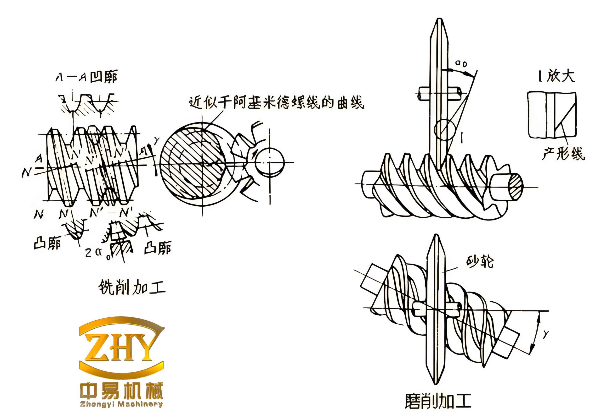
The worm gear pair achieves line contact at each meshing instant. The contact lines are smooth curves that sweep across the roller surfaces as rotation proceeds. The inclination angle γ plays a crucial role in determining the lubrication angle and self-rotation angle, both of which are key indicators of meshing quality. In the following sections, we construct a mathematical model to describe the geometry and kinematics of this system.
3. Mathematical Model
3.1 Coordinate Systems
We define the following coordinate systems based on standard gear meshing theory (see Figure 2 in the original work):
- Fixed coordinate system \(S_{1′}(O_{1′}; i_{1′}, j_{1′}, k_{1′})\) attached to the worm housing.
- Fixed coordinate system \(S_{2′}(O_{2′}; i_{2′}, j_{2′}, k_{2′})\) attached to the worm wheel housing.
- Moving coordinate system \(S_1(O_1; i_1, j_1, k_1)\) rigidly attached to the worm.
- Moving coordinate system \(S_2(O_2; i_2, j_2, k_2)\) rigidly attached to the worm wheel.
- Local roller coordinate systems \(S_{0r}(O_{0r}; i_{0r}, j_{0r}, k_{0r})\) and \(S_{0l}(O_{0l}; i_{0l}, j_{0l}, k_{0l})\) at the top centers of the right and left rollers, respectively.
- Moving frames \(S_{pr}(O_{pr}; e_{1r}, e_{2r}, n_r)\) and \(S_{pl}(O_{pl}; e_{1l}, e_{2l}, n_l)\) attached to the contact points on the right and left roller surfaces.
The initial positions are defined with \(\varphi_1 = \varphi_2 = 0\). The worm rotates by angle \(\varphi_1\) and the worm wheel by \(\varphi_2\), with the transmission ratio \(i_{12} = \omega_1/\omega_2 = z_2/z_1 = 1/i_{21}\). The coordinates of the roller centers in \(S_2\) are given as \((a_{2r}, b_{2r}, 0)\) for the right roller and \((a_{2l}, b_{2l}, 0)\) for the left roller.
3.2 Coordinate Transformations
The transformation matrix from the worm moving frame \(S_1\) to the worm wheel moving frame \(S_2\) is:
$$
M_{21} = \begin{bmatrix}
-\cos\varphi_1\cos\varphi_2 & \sin\varphi_1\cos\varphi_2 & -\sin\varphi_2 & A\cos\varphi_2 \\
\cos\varphi_1\sin\varphi_2 & -\sin\varphi_1\sin\varphi_2 & -\cos\varphi_2 & -A\sin\varphi_2 \\
-\sin\varphi_1 & -\cos\varphi_1 & 0 & 0 \\
0 & 0 & 0 & 1
\end{bmatrix}
$$
The transformation from the worm fixed frame to the worm moving frame is:
$$
M_{1’1} = \begin{bmatrix}
\cos\varphi_1 & -\sin\varphi_1 & 0 & 0 \\
\sin\varphi_1 & \cos\varphi_1 & 0 & 0 \\
0 & 0 & 1 & 0 \\
0 & 0 & 0 & 1
\end{bmatrix}
$$
Similarly, the transformation from the worm wheel fixed frame to its moving frame is:
$$
M_{2’2} = \begin{bmatrix}
\cos\varphi_2 & -\sin\varphi_2 & 0 & 0 \\
\sin\varphi_2 & \cos\varphi_2 & 0 & 0 \\
0 & 0 & 1 & 0 \\
0 & 0 & 0 & 1
\end{bmatrix}
$$
3.3 Roller Surface Representation
The parametric equations of the right roller cylindrical surface in its local coordinate system \(S_{0r}\) are:
$$
\mathbf{r}_{0r} = \begin{bmatrix} x_{0r} \\ y_{0r} \\ z_{0r} \end{bmatrix} = \begin{bmatrix} R\cos\theta_r \\ R\sin\theta_r \\ u_r \end{bmatrix}
$$
For the left roller:
$$
\mathbf{r}_{0l} = \begin{bmatrix} x_{0l} \\ y_{0l} \\ z_{0l} \end{bmatrix} = \begin{bmatrix} R\cos\theta_l \\ R\sin\theta_l \\ u_l \end{bmatrix}
$$
where \(R\) is the roller radius, \(\theta_r, \theta_l\) are circumferential parameters, and \(u_r, u_l\) are axial parameters.
3.4 Relative Velocities and Angular Velocities
Let the angular velocity of the worm be \(\boldsymbol{\omega}_1 = \omega_1 \mathbf{k}_1\). Setting \(\omega_1 = 1\) rad/s without loss of generality, we have:
$$
\boldsymbol{\omega}_1 = -\sin\varphi_2 \mathbf{i}_2 – \cos\varphi_2 \mathbf{j}_2
$$
$$
\boldsymbol{\omega}_2 = i_{21} \mathbf{k}_2
$$
The relative angular velocity is:
$$
\boldsymbol{\omega}_{12} = \boldsymbol{\omega}_1 – \boldsymbol{\omega}_2 = -\sin\varphi_2 \mathbf{i}_2 – \cos\varphi_2 \mathbf{j}_2 – i_{21} \mathbf{k}_2
$$
The position vectors of the contact points in the worm wheel frame are:
$$
\mathbf{r}_{2r} = (a_{2r} – y_{0r}\sin\gamma – z_{0r}\cos\gamma)\mathbf{i}_2 + (b_{2r} + y_{0r}\cos\gamma – z_{0r}\sin\gamma)\mathbf{j}_2 + x_{0r}\mathbf{k}_2
$$
$$
\mathbf{r}_{2l} = (a_{2l} – y_{0l}\sin\gamma – z_{0l}\cos\gamma)\mathbf{i}_2 + (b_{2l} + y_{0l}\cos\gamma – z_{0l}\sin\gamma)\mathbf{j}_2 + x_{0l}\mathbf{k}_2
$$
The relative velocities \(\mathbf{v}_{12r}\) and \(\mathbf{v}_{12l}\) are derived from the fundamental equation:
$$
\mathbf{v}_{12} = \frac{d\boldsymbol{\xi}}{dt} + \boldsymbol{\omega}_{12} \times \mathbf{r}_1 – \boldsymbol{\omega}_2 \times \boldsymbol{\xi}
$$
Since the center distance \(A\) is constant, \(d\boldsymbol{\xi}/dt = 0\). After calculation, the components of \(\mathbf{v}_{12r}\) in \(S_2\) are:
$$
\begin{aligned}
v_{12r}^x &= y_{2r} i_{21} – z_{2r} \cos\varphi_2 \\
v_{12r}^y &= -x_{2r} i_{21} + z_{2r} \sin\varphi_2 \\
v_{12r}^z &= x_{2r} \cos\varphi_2 – y_{2r} \sin\varphi_2 – A
\end{aligned}
$$
Similar expressions hold for the left roller. These velocities are then projected onto the moving frames \(S_{pr}\) and \(S_{pl}\) to obtain the components \(v_{12r1}, v_{12r2}, v_{12rn}\) and their left counterparts.
4. Meshing Analysis
4.1 Meshing Function and Equation
The condition for meshing is that the relative velocity at the contact point is orthogonal to the common normal: \(\mathbf{v}_{12} \cdot \mathbf{n} = 0\). For the right roller, this yields the meshing function:
$$
\Phi_r = v_{12rn} = M_{1r}\cos\varphi_2 + M_{2r}\sin\varphi_2 + M_{3r}
$$
where
$$
\begin{aligned}
M_{1r} &= a_{2r}\cos\theta_r – u_r\cos\gamma\cos\theta_r \\
M_{2r} &= u_r\sin\gamma\cos\theta_r – b_{2r}\cos\theta_r \\
M_{3r} &= i_{21}u_r\sin\theta_r – A\cos\theta_r – b_{2r}i_{21}\sin\gamma\sin\theta_r – a_{2r}i_{21}\cos\gamma\sin\theta_r
\end{aligned}
$$
The meshing equation is \(\Phi_r = 0\). Similarly, for the left roller:
$$
\Phi_l = M_{1l}\cos\varphi_2 + M_{2l}\sin\varphi_2 + M_{3l} = 0
$$
4.2 Contact Lines
For a fixed worm wheel rotation angle \(\varphi_2\), the instantaneous contact line on the roller surface is obtained by combining the roller surface equation with the meshing equation. For the right roller:
$$
\begin{cases}
\mathbf{r}_{0r} = [R\cos\theta_r,\; R\sin\theta_r,\; u_r]^T \\
u_r = \dfrac{P_{3r}}{P_{4r}} \\
P_{3r} = b_{2r}\sin\varphi_2\cos\theta_r + b_{2r}i_{21}\sin\gamma\sin\theta_r + a_{2r}i_{21}\cos\gamma\sin\theta_r + A\cos\theta_r – a_{2r}\cos\varphi_2\cos\theta_r \\
P_{4r} = \sin\gamma\sin\varphi_2\cos\theta_r + i_{21}\sin\theta_r – \cos\gamma\cos\varphi_2\cos\theta_r
\end{cases}
$$
For the left roller, similar equations hold with subscript \(l\). The contact lines are smooth curves that transform from near-straight lines at the entry and exit zones to denser lines near the worm throat.
4.3 Tooth Surface Equations
The worm tooth surface is generated by the family of contact lines as \(\varphi_2\) varies. The right tooth surface equation in the worm coordinate system \(S_1\) is:
$$
\begin{cases}
x_{1r} = y_{2r}\cos\varphi_1\sin\varphi_2 – x_{2r}\cos\varphi_1\cos\varphi_2 – z_{2r}\sin\varphi_1 + A\cos\varphi_1 \\
y_{1r} = x_{2r}\sin\varphi_1\cos\varphi_2 – y_{2r}\sin\varphi_1\sin\varphi_2 – z_{2r}\cos\varphi_1 – A\sin\varphi_1 \\
z_{1r} = -x_{2r}\sin\varphi_2 – y_{2r}\cos\varphi_2 \\
\varphi_2 \in [-\pi/5,\; \pi/5]
\end{cases}
$$
The left tooth surface is defined analogously.
5. Performance Parameters
5.1 Induced Normal Curvature
The induced normal curvature along the common normal direction of the contact line is a measure of contact conformity. Using the moving frame method, the induced curvature for the right side is:
$$
k_{12\sigma r} = -k_{21\sigma r} = -\frac{(v_{12r1}/R – \omega_{122r})^2 + (\omega_{121r})^2}{\Psi_r}
$$
where \(\Psi_r\) is the boundary function, and \(\omega_{121r}, \omega_{122r}\) are projections of the relative angular velocity onto the moving frame. The results for a typical set of parameters are summarized in Table 1.
| \(\varphi_2\) (rad) | Right roller \(k_{12\sigma r}\) (1/mm) | Left roller \(k_{12\sigma l}\) (1/mm) |
|---|---|---|
| -0.628 | 0.00185 | 0.00172 |
| -0.314 | 0.00160 | 0.00155 |
| 0 | 0.00142 | 0.00148 |
| 0.314 | 0.00135 | 0.00152 |
| 0.628 | 0.00128 | 0.00160 |
The induced curvatures are small and vary only slightly across the meshing cycle, indicating good contact conformity. The right roller shows slightly lower values than the left, implying better conformity on the right side.
5.2 Lubrication Angle
The lubrication angle \(\mu\) is defined as the angle between the relative velocity vector and the contact line tangent. A larger lubrication angle (closer to 90°) improves lubricant film formation. The lubrication angle for the right roller is:
$$
\mu_r = \arcsin\left(\frac{|v_{12r1}(v_{12r1}/R – \omega_{122r}) + v_{12r2}\omega_{121r}|}{\sqrt{(v_{12r1}/R – \omega_{122r})^2 + (\omega_{121r})^2}\sqrt{v_{12r1}^2 + v_{12r2}^2}}\right)
$$
Table 2 presents computed lubrication angles.
| \(\varphi_2\) (rad) | Right \(\mu_r\) (°) | Left \(\mu_l\) (°) |
|---|---|---|
| -0.628 | 88.2 | 89.3 |
| -0.314 | 88.8 | 89.5 |
| 0 | 88.5 | 89.0 |
| 0.314 | 87.9 | 88.6 |
| 0.628 | 87.6 | 88.4 |
The lubrication angles are all above 87.5°, indicating excellent lubricating conditions. The left roller consistently provides slightly higher angles than the right roller.
5.3 Self-Rotation Angle
The self-rotation angle \(\mu_{z}\) is the angle between the relative velocity and the roller axis. A value close to 90° means the roller can rotate freely with minimal resistance. For the right roller:
$$
\mu_{zr} = \arccos\left(\frac{|\mathbf{k}_{0r} \cdot \mathbf{v}_{12r}|}{|\mathbf{v}_{12r}|}\right)
$$
Table 3 lists the results.
| \(\varphi_2\) (rad) | Right \(\mu_{zr}\) (°) | Left \(\mu_{zl}\) (°) |
|---|---|---|
| -0.628 | 89.1 | 89.8 |
| -0.314 | 89.3 | 89.9 |
| 0 | 88.9 | 89.5 |
| 0.314 | 88.6 | 89.2 |
| 0.628 | 88.5 | 89.1 |
The self-rotation angles are all above 88.5°, confirming that the rollers can rotate easily, minimizing sliding friction.
5.4 Relative Entrainment Velocity
The relative entrainment velocity \(v_{jx}\) is half the sum of the velocities of the two surfaces along the common normal direction. It influences the formation of an elastohydrodynamic oil film. The formula for the right side is:
$$
v_{jxr} = \frac{v_{1\sigma r} + v_{2\sigma r}}{2}
$$
where
$$
\begin{aligned}
v_{1\sigma r} &= \frac{v_{1r1}(v_{12r1}/R – \omega_{122r}) + v_{1r2}\omega_{121r}}{T_r} \\
v_{2\sigma r} &= \frac{v_{2r1}(v_{12r1}/R – \omega_{122r}) + v_{2r2}\omega_{121r}}{T_r} \\
T_r &= \sqrt{(v_{12r1}/R – \omega_{122r})^2 + (\omega_{121r})^2}
\end{aligned}
$$
Computed values are given in Table 4.
| \(\varphi_2\) (rad) | Right \(v_{jxr}\) (m/s) | Left \(v_{jxl}\) (m/s) |
|---|---|---|
| -0.628 | 0.82 | 0.85 |
| -0.314 | 0.75 | 0.79 |
| 0 | 0.68 | 0.72 |
| 0.314 | 0.72 | 0.76 |
| 0.628 | 0.80 | 0.83 |
The entrainment velocities exhibit a parabolic trend with a minimum near the throat region. The left roller shows slightly higher values, which benefits oil film formation.
6. Conclusion
We have presented a comprehensive theoretical analysis of the parallel inclined double roller enveloping hourglass worm gear. The main contributions are as follows:
- The structural principle and geometric configuration of the novel worm gear were described in detail.
- Using spatial meshing theory and moving frame methods, we derived the complete mathematical model, including coordinate transformations, relative velocity expressions, meshing equations, contact line equations, and tooth surface equations.
- Key performance parameters—induced normal curvature, lubrication angle, self-rotation angle, and relative entrainment velocity—were computed. Numerical results show that the induced curvature is small (below 0.002 1/mm), indicating good contact conformity. Lubrication angles exceed 87.5°, self-rotation angles exceed 88.5°, and entrainment velocities are adequate for oil film formation.
- The analysis confirms that the proposed worm gear drive exhibits excellent meshing performance, combining low friction, good lubrication, and high load capacity. This design is promising for high-precision and high-efficiency transmission applications.