
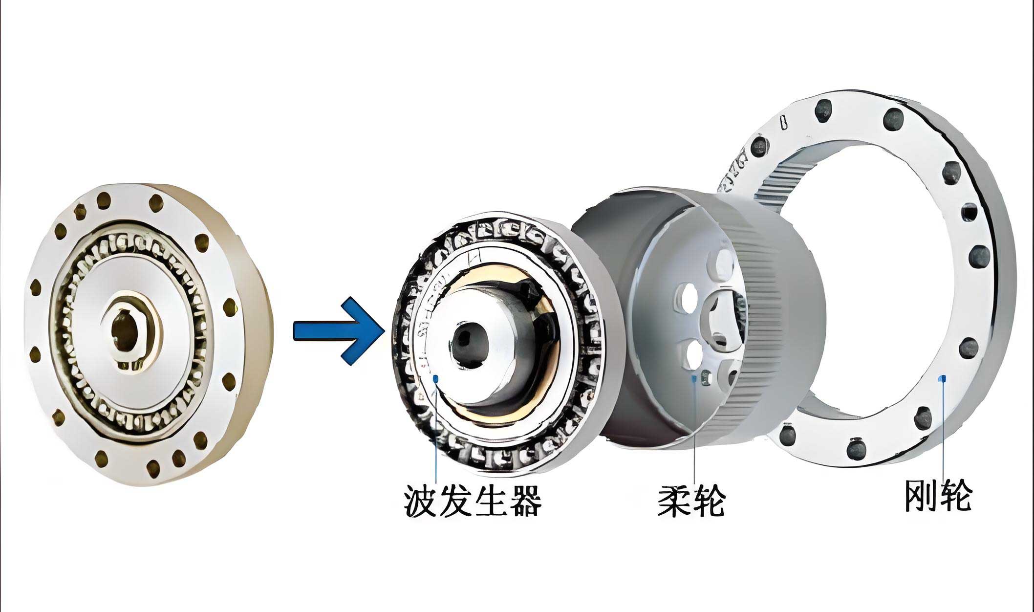
Strain wave gearing, also commonly referred to as harmonic drive, is a pivotal technology in precision motion control. Its unique combination of high reduction ratios, compactness, zero-backlash characteristics, and high torque capacity makes it indispensable in applications ranging from industrial robots and aerospace mechanisms to semiconductor manufacturing equipment. The core assembly consists of three primary components: a rigid, internally-toothed Circular Spline (CS), a flexible, externally-toothed Flexspline (FS), and an elliptical Wave Generator (WG) that deforms the Flexspline to create a rotating mesh pattern. Despite the inherent zero-backlash design, these transmissions are not free from positioning inaccuracies. A critical performance metric, the Angular Transmission Error (ATE), directly limits the static positioning precision of systems, particularly in semi-closed loop control configurations where only the motor position is directly measured.
The Angular Transmission Error is defined as the deviation between the actual output position and the ideal position dictated by the input and the gear ratio. Mathematically, it is expressed as:
$$ \theta_{TE} = \theta_L – \frac{\theta_M}{N} $$
where \( \theta_{TE} \) is the angular transmission error, \( \theta_L \) is the load-side angular displacement, \( \theta_M \) is the motor-side angular displacement, and \( N \) is the reduction ratio of the strain wave gear.
To effectively address and compensate for this error, it is essential to decompose it into its constituent physical origins. Our analysis identifies two dominant, separable components that constitute the total ATE in a strain wave gear: a synchronous component and a nonlinear elastic (hysteretic) component. This decomposition forms the foundation for an accurate predictive model and an effective compensation strategy.
1. Mathematical Modeling of the Synchronous Error Component
The synchronous component of the transmission error, denoted as \( \theta_{Sync} \), is periodic with respect to the rotation of the gear elements. This error arises from inherent manufacturing imperfections such as tooth profile errors, pitch deviations of the Flexspline and Circular Spline, and assembly misalignments (e.g., eccentricity). Its key characteristic is that its waveform repeats every cycle of the motor shaft or wave generator rotation.
Since this component is fundamentally periodic, it can be effectively modeled as a Fourier series expansion of the motor angle. In a semi-closed loop system, the motor angle \( \theta_M \) is the directly measured quantity, making it the most practical reference for modeling. Therefore, the synchronous error is represented as:
$$ \theta_{Sync} = \sum_{i=1}^{n_M} A_M(i) \cos\left( i \cdot \theta_{M} + \phi_M(i) \right) $$
Here, \( i \) is the harmonic order, \( A_M(i) \) is the amplitude of the \( i \)-th harmonic (typically in arcseconds), and \( \phi_M(i) \) is its corresponding phase shift. The dominant harmonics are often low-order (e.g., 1st, 2nd, 4th), corresponding to once-per-revolution errors and their multiples.
Experimental identification involves measuring the ATE over several complete revolutions of the motor under low-speed, quasi-static conditions to avoid dynamic effects. A spectral analysis (FFT) of the recorded error data reveals the significant harmonic amplitudes and phases, which are then tabulated for the model. A representative parameter set derived from such an analysis is summarized below.
| Harmonic Order, \( i \) | Amplitude, \( A_M(i) \) [arcsec] | Phase, \( \phi_M(i) \) [deg] |
|---|---|---|
| 1 | 4.90 | -126.8 |
| 2 | 9.33 | -132.1 |
| 3 | 2.09 | -96.2 |
| 4 | 12.21 | 105.7 |
| 6 | 3.18 | -127.0 |
| 8 | 1.87 | 124.3 |
2. Mathematical Modeling of the Nonlinear Elastic (Hysteretic) Error Component
The second major component, the nonlinear elastic error \( \theta_{Hys} \), is a non-periodic phenomenon primarily observed during micro-motions and at velocity reversals. It stems from the complex, nonlinear elastic deformation of the Flexspline’s thin-walled structure and the friction in the moving interfaces (e.g., between the wave generator bearing and the Flexspline cup). This component exhibits pronounced hysteresis, meaning the error path during forward motion differs from that during reverse motion, creating a closed loop.
This behavior is analogous to the rolling friction or presliding displacement observed in mechanical contacts with nonlinear stiffness. To model this, we adopt a hysteresis modeling framework. The error depends on the direction of motion \( \operatorname{sgn}(\omega_M) \) and the magnitude of elastic deflection \( \delta \) since the last velocity reversal. The model is defined piecewise:
$$ \theta_{Hys} = \begin{cases}
\operatorname{sgn}(\omega_M) \left[ 2\theta_{offset} \cdot g(\xi) – \theta’_{Hys} \right] & \text{if } |\delta| < \theta_r \text{ and } |\theta_{Hys}| < \theta_{offset} \\
\operatorname{sgn}(\omega_M) \cdot \theta_{offset} & \text{if } |\delta| \geq \theta_r \text{ or } |\theta_{Hys}| \geq \theta_{offset}
\end{cases} $$
where the shape function \( g(\xi) \) governs the transition within the hysteresis loop:
$$ g(\xi) = \begin{cases}
\frac{1}{2-n} \left[ \xi^{n-1} – (n-1)\xi \right] & \text{for } n \neq 2 \\
\xi (1 – \ln \xi) & \text{for } n = 2
\end{cases} $$
The key model parameters are:
- \( \delta = |\theta_M – \delta_0 | \): The absolute angular displacement from the reversal point \( \delta_0 \).
- \( \xi = \delta / \theta_r \): The normalized displacement.
- \( \theta_r \): The “reversal radius” or the angular displacement within which the hysteresis loop is active.
- \( \theta_{offset} \): The saturation value of the hysteretic error.
- \( n \): A shape parameter controlling the width of the hysteresis loop.
- \( \theta’_{Hys} \): The error value at the previous calculation step (introducing memory).
This model captures the essential features: a linear-like elastic region for very small motions, a smooth transition to a saturated frictional plateau, and a directional dependence that creates the loop. The parameters \( \theta_r \), \( \theta_{offset} \), and \( n \) are identified through experiments involving low-frequency, small-amplitude sinusoidal excitations and observing the resulting Lissajous plots of ATE versus motor angle.
| Parameter | Symbol | Value | Unit |
|---|---|---|---|
| Reversal Radius | \( \theta_r \) | 20 | deg |
| Error Saturation | \( \theta_{offset} \) | 40 | arcsec |
| Shape Factor | \( n \) | 1.6 | – |
3. Model Validation and Experimental Verification
The complete ATE model, combining both components, is given by:
$$ \theta_{TE} = \theta_{Sync}(\theta_M) + \theta_{Hys}(\theta_M, \omega_M, \delta_0) $$
Validation of this composite model is critical. Experiments are conducted on a test bench equipped with a high-resolution encoder on the load side to measure the true ATE. The motor is commanded to follow specific trajectories, such as large slow rotations (to highlight \( \theta_{Sync} \)) and small-amplitude low-frequency sinusoids (to highlight \( \theta_{Hys} \)).
The results demonstrate excellent agreement between the model prediction and experimental measurements. For the synchronous component, the predicted waveform based on the Fourier series closely matches the periodic error measured over multiple revolutions. For the hysteretic component, the model accurately reproduces the distinctive looping behavior in the ATE vs. motor angle plot during reciprocating micro-motions. The model’s ability to predict both the periodic ripples and the directional lag confirms its validity as a comprehensive descriptor of strain wave gear error phenomena.
4. Feedforward Compensation Strategy and Performance Evaluation
The primary application of the high-fidelity ATE model is model-based feedforward compensation. In a semi-closed loop system, the controller only knows the motor position \( \theta_M \). The goal is to calculate a compensating motor command \( \theta_{M,cmd}^* \) that, after the distortion introduced by the strain wave gear, results in the desired load position \( \theta_{L,des} \).
The compensation is implemented as follows. For a desired load movement corresponding to a nominal motor movement of \( \theta_{M,des} = N \cdot \theta_{L,des} \), the controller first uses the real-time model to predict the ATE that would occur:
$$ \hat{\theta}_{TE} = \theta_{Sync}(\theta_{M,des}) + \theta_{Hys}(\theta_{M,des}, \omega_{M,des}, \text{state}) $$
This predicted error is then subtracted from the nominal command to generate the compensated motor command:
$$ \theta_{M,cmd}^* = \theta_{M,des} – N \cdot \hat{\theta}_{TE} $$
By injecting this modified command, the inherent error of the strain wave gear is effectively canceled out in the feedforward path.
To quantify the performance improvement, a static positioning test is performed. The system is commanded to execute a sequence of small step motions (micro-steps). Without compensation, the load position exhibits significant steady-state scatter around the target due to the uncompensated ATE, particularly the hysteretic component which is not rejected by the feedback loop. The effectiveness of different compensation schemes is evaluated by statistically analyzing this steady-state scatter, often characterized by the 3σ value (three times the standard deviation).
| Compensation Scheme | Steady-State Scatter (3σ) | Normalized Scatter (%) | Mean Error [arcsec] |
|---|---|---|---|
| No Compensation | 75.0 arcsec | 100.0% | 34.2 |
| Synchronous Error Only | 50.2 arcsec | 66.9% | 29.0 |
| Hysteretic Error Only | 55.7 arcsec | 74.2% | -23.2 |
| Full Model (Sync + Hys) | 30.2 arcsec | 40.2% | -29.2 |
The results are decisive. While compensating for only the synchronous or only the hysteretic component provides some improvement, the full composite model delivers the highest performance. The implementation of the complete ATE model as a feedforward compensator reduced the steady-state positioning scatter by approximately 60% (from 75.0 arcsec to 30.2 arcsec). This dramatic reduction directly translates to a significant enhancement in the static positioning accuracy and repeatability of systems employing strain wave gears.
5. Conclusion and Outlook
This work has presented a comprehensive methodology for modeling and compensating the angular transmission error in strain wave gears. By physically decomposing the total error into a synchronous, periodic component and a nonlinear elastic, hysteretic component, we established accurate mathematical models for each. The synchronous model employs a Fourier series based on motor angle, while the hysteretic model uses a nonlinear framework inspired by rolling friction to capture directional effects and saturation.
Experimental validation confirmed the model’s fidelity in predicting both error types. The integration of this composite model into a feedforward compensation strategy for semi-closed loop control systems proved highly effective. The key outcome was a reduction of steady-state positioning scatter by about 60%, which corresponds to a 40% residual of the original uncompensated error, thereby substantially improving the static positioning precision of the drivetrain.
Future work may focus on the adaptive identification of model parameters under varying load and temperature conditions, as these factors can influence the nonlinear stiffness and friction within the strain wave gear. Furthermore, integrating this feedforward compensator with advanced feedback control strategies, such as robust or adaptive control, could address residual errors and disturbances, pushing the performance boundaries of precision systems utilizing strain wave gearing technology even further.