
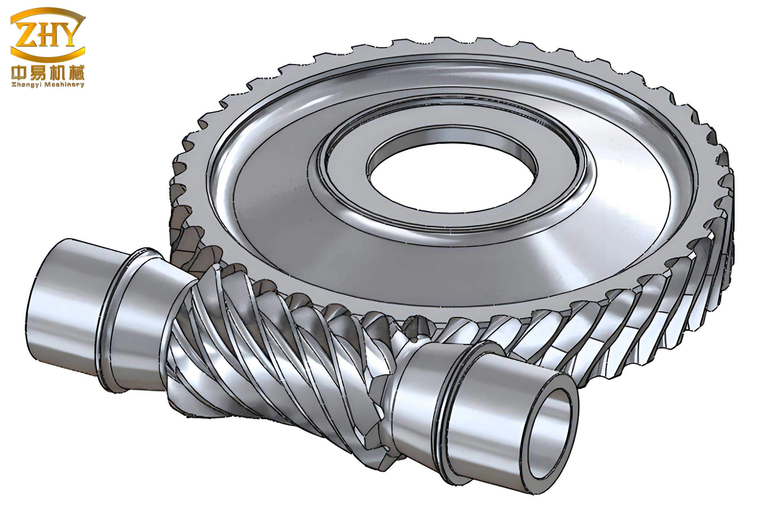
The design and analysis of screw gear systems, encompassing the worm and the worm wheel, traditionally involve a meticulous and iterative process. Each modification to a fundamental parameter, such as the module, number of threads, or pressure angle, necessitates a complete re-evaluation of dependent dimensions and often a full rebuild of the 3D model. This approach is not only time-consuming but also prone to human error, significantly extending the product development cycle. To overcome these challenges, I have developed and implemented a comprehensive methodology for the parametric design and motion simulation of screw gears within the Siemens NX (UG) software environment. This approach leverages the power of parametric modeling and expression-driven design to create dynamic, intelligent models that update automatically with changes to core parameters, thereby streamlining the entire design process.
The core of this methodology lies in utilizing UG’s “Expressions” functionality. Expressions are algebraic and conditional statements that define the relationships between different parameters of a model. By establishing these relationships at the outset, the model becomes fully parametric. This means that altering a primary driving parameter, like the module (m), automatically triggers the recalculation of all associated dimensions—such as pitch diameters, addendum, dedendum, and center distance—and subsequently updates the entire 3D geometry. This dynamic linking is the cornerstone of efficient design iteration and customization.
1. Foundational Parameters and Mathematical Framework
The first step in any parametric design is to define the complete set of independent (input) and dependent (calculated) parameters. For an involute screw gear set, the fundamental parameters are established, and their interrelationships are encoded using mathematical formulas. The table below summarizes the primary parameters, their symbols, defining equations, and typical initial values used as a starting point for the design.
| Parameter Name | Symbol | Formula / Definition | Initial Value |
|---|---|---|---|
| Module | $$m$$ | Primary size parameter | 2 mm |
| Pressure Angle | $$\alpha$$ | Standard tooth profile angle | 20° |
| Number of Worm Wheel Teeth | $$Z_2$$ | – | 36 |
| Addendum Coefficient | $$h_a^*$$ | $$h_a = h_a^* \cdot m$$ | 1 |
| Dedendum/Clearance Coefficient | $$c^*$$ | $$c = c^* \cdot m$$ | 0.25 |
| Worm Wheel Pitch Diameter | $$d_2$$ | $$d_2 = m \cdot Z_2$$ | 72 mm |
| Worm Wheel Base Diameter | $$d_{b2}$$ | $$d_{b2} = d_2 \cdot \cos(\alpha)$$ | 67.66 mm |
| Worm Wheel Tip Diameter | $$d_{a2}$$ | $$d_{a2} = m \cdot (Z_2 + 2h_a^*)$$ | 76 mm |
| Worm Wheel Root Diameter | $$d_{f2}$$ | $$d_{f2} = m \cdot (Z_2 – 2h_a^* – 2c^*)$$ | 67 mm |
| Worm Wheel Face Width | $$B$$ | Design choice based on strength | 30 mm |
| Number of Worm Threads (Starts) | $$Z_1$$ | – | 3 |
| Worm Diameter Factor | $$q$$ | $$q = d_1 / m$$ | 13 |
| Worm Pitch Diameter | $$d_1$$ | $$d_1 = m \cdot q$$ | 26 mm |
| Lead Angle of Worm | $$\gamma$$ | $$\gamma = \arctan\left(\frac{Z_1}{q}\right)$$ | 12.994° |
| Helix Angle of Worm Wheel | $$\beta$$ | $$\beta = \gamma$$ (for crossed-axis mesh) | 12.994° |
| Center Distance | $$a$$ | $$a = \frac{m}{2} (q + Z_2)$$ | 49 mm |
These parameters and formulas are input directly into the UG Expressions dialog box. This action creates a centralized parameter table that governs the entire screw gear assembly model. For instance, the expression for the worm wheel tip diameter would be entered as `da = m * (Z2 + 2*ha_star)`. UG treats these not as static numbers but as live variables.
2. Parametric Modeling of the Worm Wheel
The construction of the worm wheel is a multi-step process that heavily relies on law curves defined by parametric equations.
2.1 Generating the Involute Tooth Profile
The tooth profile in a plane normal to the axis is an involute curve. This curve is generated using UG’s “Law Curve” tool. The parametric equations for an involute derived from a base circle of diameter $$d_b$$ are defined with a parameter `t` ranging from 0 to 1.
For a given roll angle `u` (in degrees) derived from `t`, the corresponding arc length `s` on the base circle is:
$$ u = 60 \cdot t $$
$$ s = \frac{\pi \cdot d_b \cdot t}{4} $$
The coordinates for one side of the symmetric involute are:
$$ x_t = \frac{d_b}{2} \cos(u) + s \cdot \sin(u) $$
$$ y_t = \frac{d_b}{2} \sin(u) – s \cdot \cos(u) $$
$$ z_t = 0 $$
The opposing flank’s coordinates are simply `(x_t, -y_t, 0)`. Inputting these equations via the “Law Curve” function creates the precise involute curves. These curves, along with the tip, root, and pitch circles sketched in a datum plane, form the closed 2D profile of a single tooth space, which is then filleted at the root for strength.
2.2 Defining the Helical Tooth Path
The worm wheel teeth are helical, wrapping around the axis with a lead angle $$\beta$$. This three-dimensional path is also created as a law curve. The law defines a helical path along the face width `B` of the wheel. One such equation for the guiding helix is:
$$ x_h = a – B \cdot \cos(60 \cdot t) $$
$$ y_h = -B \cdot \tan(\gamma) \cdot t $$
$$ z_h = B \cdot t $$
where `a` is the center distance. This curve dictates the sweep path for the tooth profile.
2.3 Creating the 3D Worm Wheel Body
With the 2D tooth space profile and the 3D helical path defined, the “Sweep” command is used. The profile is swept along the helical guide curve, resulting in a solid helical groove—the negative space of one tooth. This single groove feature is then patterned circularly around the wheel axis with an angular pitch of $$360^\circ / Z_2$$, creating all tooth spaces simultaneously. Finally, standard features like the hub, web, and keyway are added parametrically, with their dimensions linked to the primary gear parameters (e.g., bore diameter linked to `d_f2`). The resulting model is a fully parametric worm wheel; changing `Z_2` to 24 instantly regenerates a new model with 24 accurately spaced teeth.
3. Parametric Modeling of the Worm
The modeling of the worm is conceptually similar but involves defining the thread profile in an axial section. The profile is often trapezoidal, approximating the shape of the worm wheel tooth space.
Key parameters specific to the worm, such as the thread tip radius (`rt`), root radius, and detailed involute parameters for the flank (if modeled precisely), are added to the Expressions list. The core sweep operation for creating the helical thread uses a law that defines a twist angle proportional to the length and lead:
$$ \theta = t \cdot \left[ \frac{H \cdot \tan(\gamma)}{r_p} \right] \text{ (in radians)} $$
where `H` is the worm length and `r_p` is a reference radius. A 2D thread profile is swept along the worm’s axial length with this angular law, creating one helical thread. This thread is then patterned around the axis $$Z_1$$ times to create a multi-start screw gear. The worm body (cylindrical blanks at the tip and root diameters) is created and combined with the threaded section via Boolean operations. As with the wheel, every dimension is controlled by the master expressions.
4. Dynamic Model Update and Design Iteration
The true power of this parametric framework is realized during design iteration. Suppose the initial design with `m=2`, `Z2=36`, and `Z1=3` requires a higher torque capacity. The engineer decides to increase the module to `m=3` and reduce the wheel size to `Z2=24` while keeping the center distance roughly similar by adjusting `q`. The designer simply opens the Expressions window, changes these three primary values (`m`, `Z2`, `q`), and confirms the change.
UG’s software automatically recalculates every dependent expression: new pitch diameters, new tip and root diameters, a new center distance, a new lead angle, and all associated law curve equations. It then automatically regenerates the entire 3D assembly—both the worm and the worm wheel—to reflect these new dimensions. The tooth count updates, the helix angles change, and the meshing geometry adjusts correctly, all within seconds. This process eliminates hours of manual remodeling and recalculation, fundamentally accelerating the design cycle for the screw gear system.
5. Motion Simulation and Interference Analysis
Creating an accurate 3D model is only part of the validation. Ensuring that the screw gear pair meshes correctly without interference and moves as intended is critical. UG’s integrated Motion Simulation module is used for this virtual prototyping.
- Assembly & Environment: The parametrically modeled worm and wheel are assembled with the correct center distance `a`. A new motion simulation file is created.
- Defining Links: The worm and the worm wheel are defined as two rigid links (e.g., Link_Worm, Link_Wheel).
- Applying Joints: A rotational joint is applied to the worm, fixing its axis of rotation. Another rotational joint is applied to the worm wheel, fixing its axis, which is perpendicular and offset from the worm’s axis. The worm joint is assigned a driver, say 360 deg/sec, defining it as the input.
- Creating a Gear Coupling: A “Gear Coupling” joint (or a 3D Contact force) is established between the two rotational joints. The transmission ratio is defined by the ratio of teeth: $$ i = \frac{Z_2}{Z_1} = 12 $$. This ensures the worm wheel rotates at 1/12th the speed of the worm.
- Setting Up Interference Check: This is a crucial step. The “Interference” analysis tool is configured. The worm and worm wheel are selected as the two sets of bodies to check. The option “Highlight on Interference” is chosen. This instructs the solver to stop the simulation and vividly color any penetrating volumes if contact geometry is incorrect.
- Solving and Analyzing: The solver runs the simulation for a set time (e.g., 20 seconds). The designer can animate the model, observing the smooth (or problematic) meshing of the screw gear teeth throughout the engagement. If the parametric design is correct, the motion will be smooth, and no interference highlights will appear. If an error existed in the profile or helix angle definition, the interference check would immediately flag it, allowing for correction in the master expressions before any physical prototype is made.
6. Conclusion and Broader Implications
The integration of parametric modeling via expressions and dynamic motion simulation within UG software presents a robust and efficient methodology for screw gear design. This approach transforms the design process from a static, sequential task into a dynamic, iterative exploration. The major benefits are:
- Dramatically Increased Efficiency: Design changes that once took hours or days are executed in minutes.
- Inherent Consistency and Accuracy: Mathematical relationships ensure all dimensions are always synchronized, eliminating manual calculation errors.
- Enhanced Validation: Virtual motion simulation with interference checking provides high-confidence validation early in the design phase, reducing prototyping costs and time.
- Foundation for Knowledge Reuse: The parametric model serves as a template. By saving different sets of expression values, a library of standardized screw gear designs can be created, facilitating rapid configuration of new products.
While demonstrated here for screw gears, this paradigm of expression-driven parametric design coupled with simulation is directly applicable and highly valuable for a wide range of mechanical components, including various gear types (spur, helical, bevel), bearings, cams, and linkages. It embodies a modern, digital approach to mechanical design that is essential for competitiveness in today’s engineering landscape, ensuring both precision and agility in product development.