
I present a unified study of the design theory and gear machining method for bevel gears whose meshing contact remains purely rolling over the entire contact path. Traditional bevel gears operate with mixed rolling and sliding contact. Sliding contact is not merely an efficiency loss; it is a direct source of scuffing, micropitting, thermal imbalance, and edge stress concentration. My starting point is therefore not the classical envelope of a generating surface, but the conjugate-curve meshing principle, in which a spatial curve and its conjugate curve control the instantaneous contact point and allow a tooth surface to be generated locally from a prescribed contact path. I derive the continuous pure-rolling condition, prove the uniqueness of the conjugate curve, construct the tooth surface from the normal section, analyze the second-order contact properties, optimize the surface by presetting a parabolic transmission error, and finally develop a digital generating gear machining method using a disc milling cutter. The numerical and experimental results show that the proposed design and gear machining route can produce a bevel gear pair whose contact trace lies near the pitch line and whose contact pattern remains in the middle of the tooth surface.
Kinematic foundation and pure-rolling contact condition. I describe the bevel gear pair by four coordinate systems: a fixed frame \(S_0\), a fixed auxiliary frame \(S_p\), and two moving frames \(S_1\) and \(S_2\) rigidly attached to the pinion and the gear. The pinion rotates about the \(z_1\) axis, while the gear rotates about the \(z_2\) axis, and the two axes intersect at the common origin. The shaft angle is \(\xi\), the pinion rotation angle is \(\phi\), and the gear rotation angle is \(\psi\). For a constant transmission ratio \(i_{21}=\omega_2/\omega_1\), I have
$$
\psi=i_{21}\phi .
$$
The transformation from \(S_1\) to \(S_0\) is
$$
M_{01}=
\begin{bmatrix}
\cos\phi & \sin\phi & 0 & 0\\
-\sin\phi & \cos\phi & 0 & 0\\
0 & 0 & 1 & 0\\
0 & 0 & 0 & 1
\end{bmatrix},
$$
and the transformation from \(S_0\) to \(S_p\) is
$$
M_{p0}=
\begin{bmatrix}
1 & 0 & 0 & 0\\
0 & \cos\xi & -\sin\xi & 0\\
0 & \sin\xi & \cos\xi & 0\\
0 & 0 & 0 & 1
\end{bmatrix}.
$$
The transformation from \(S_p\) to \(S_2\) is
$$
M_{2p}=
\begin{bmatrix}
\cos\psi & 0 & -\sin\psi & 0\\
0 & 1 & 0 & 0\\
\sin\psi & 0 & \cos\psi & 0\\
0 & 0 & 0 & 1
\end{bmatrix}.
$$
Combining these matrices gives the transformation from \(S_1\) to \(S_2\):
$$
M_{21}=M_{2p}M_{p0}M_{01}.
$$
For any candidate contact point, the relative velocity in \(S_0\) is
$$
\mathbf{v}_{12}^{(0)}
=
\boldsymbol{\omega}_{1}^{(0)}\times \mathbf{r}_{1}^{(0)}
–
\boldsymbol{\omega}_{2}^{(0)}\times \mathbf{r}_{2}^{(0)} .
$$
After transforming to \(S_1\), I write the relative velocity as
$$
\mathbf{v}_{12}^{(1)}
=
M_{10}M_{01}\mathbf{r}_{1}^{(1)}
–
M_{10}M_{02}\mathbf{r}_{2}^{(2)} .
$$
Pure rolling contact requires the sliding velocity to vanish at every instant of meshing:
$$
\mathbf{v}_{12}^{(1)}=\mathbf{0}.
$$
This condition is much stronger than the usual conjugate condition \(\mathbf{n}\cdot\mathbf{v}_{12}=0\). It forces the instantaneous contact point to lie on the pitch cone. Therefore, I parameterize the pitch cone of the pinion as
$$
\mathbf{S}_1(t,u)=
\begin{pmatrix}
p\,u\sin t\\
p\,u\cos t\\
u\\
1
\end{pmatrix},
\qquad
p=\tan\delta_1,
$$
where \(\delta_1\) is the pinion pitch angle. A general contact curve on this pitch cone is written as
$$
\mathbf{r}_1(t)=
\begin{pmatrix}
p f(t)\sin t\\
p f(t)\cos t\\
f(t)\\
1
\end{pmatrix}.
$$
The function \(f(t)\) defines the radial growth of the contact trace. For a logarithmic spiral bevel gear, I select
$$
f(t)=b e^{mt},
\qquad
n=\sin\delta_1,
\qquad
b=\cos\delta_1,
\qquad
m=n\cot\beta_k,
$$
where \(\beta_k\) is the spiral angle. Substituting this contact trace into the pure-rolling condition yields the necessary relation between the motion parameters and the pitch geometry:
$$
t=\phi,
\qquad
p=\frac{\sin\xi}{i_{21}-\cos\xi}.
$$
This result is important because it shows that the contact trace cannot be chosen arbitrarily. Once the shaft angle and transmission ratio are fixed, the pitch angle and the contact parameter are determined. The conjugate curve in the gear frame is then obtained by
$$
\mathbf{r}_2(t)=M_{21}(t)\mathbf{r}_1(t).
$$
For the logarithmic spiral case, I obtain
$$
\mathbf{r}_2(t)=
\begin{pmatrix}
e^{mt}\left(i_{21}t\sin\phi – p\cos\phi\sin\xi\right)\\
e^{mt}\left(i_{21}t\cos\phi + p\cos\phi\sin\xi\right)\\
e^{mt}\left(i_{21}t+p\cos\xi\right)\\
1
\end{pmatrix}.
$$
Uniqueness of the conjugate curve and tooth surface generation. A central question is whether a given contact trace determines a unique conjugate trace. I define the meshing function
$$
F(t,\phi)=\mathbf{n}_1(t)\cdot\mathbf{v}_{12}^{(1)}(t,\phi).
$$
The normal vector in the normal plane of the contact trace can be expressed as
$$
\mathbf{n}_1(t)=\cos\theta_1(t)\,\boldsymbol{\beta}_1(t)
+
\sin\theta_1(t)\,\boldsymbol{\gamma}_1(t),
$$
where \(\boldsymbol{\beta}_1\) and \(\boldsymbol{\gamma}_1\) are the principal normal and binormal of the contact curve, and \(\theta_1(t)\) is a continuous orientation angle. Because the contact curve is regular, the derivatives of the Frenet frame are continuous. Hence \(F(t,\phi)\) is continuously differentiable with respect to both \(t\) and \(\phi\). If
$$
\frac{\partial F}{\partial \phi}\neq 0,
$$
the implicit function theorem gives a unique continuous function
$$
\phi=g(t),
\qquad
\frac{d\phi}{dt}
=
-\frac{\partial F/\partial t}{\partial F/\partial \phi}.
$$
Therefore, for a prescribed normal direction along the contact trace, the conjugate curve is unique. This uniqueness is essential for a deterministic design and for later gear machining, because the cutter path is derived from the same conjugate geometry.
The contact curve itself is only a mathematical object. To obtain a load-carrying tooth surface, I construct a normal section at each contact point. In the local Frenet frame of the contact trace, the section curve is
$$
\mathbf{r}_{sec1}^{F_r}(u)=
\begin{pmatrix}
0\\
y(u)\\
z(u)\\
1
\end{pmatrix}.
$$
Then the pinion tooth surface is generated by moving this section along the contact trace:
$$
\mathbf{S}_1(t,u)=M_{1F_r}(t)\,\mathbf{r}_{sec1}^{F_r}(u).
$$
Similarly, the gear tooth surface is
$$
\mathbf{S}_2(t,v)=M_{2F_r}(t)\,\mathbf{r}_{sec2}^{F_r}(v).
$$
I also verify that the generated local conjugate surface does not penetrate the mating surface. The condition
$$
\mathbf{n}_1\cdot \frac{d}{dt}\left(M_{21}\mathbf{r}_1\right)=0
$$
is satisfied by the construction. Consequently, the curve-to-surface extension is not merely a geometric exercise; it produces an admissible tooth surface entity that can be used for contact analysis and for gear machining path planning.
Second-order contact analysis. I now analyze the local shape of the tooth surface near the instantaneous contact point. This is necessary because the contact ellipse, the sensitivity to misalignment, and the risk of edge contact are all controlled by second-order geometry. I express the normal vector in terms of the normal pressure angle \(\alpha_n\):
$$
\cos\left(\frac{\pi}{2}-\alpha_n\right)
=
\left\langle \mathbf{n}_1,\mathbf{r}_{rad}\right\rangle,
$$
where \(\mathbf{r}_{rad}\) is the radial unit vector along the contact trace. The normal vector must also satisfy
$$
\mathbf{n}_1\cdot \mathbf{r}_1′(t)=0,
\qquad
\mathbf{n}_1\cdot \mathbf{n}_1=1.
$$
Using a skew rectilinear coordinate system \(S_\alpha\) attached to the contact trace, I choose the covariant basis vectors
$$
\mathbf{g}_1^{(S_\alpha)}=\mathbf{r}_1′(t),
\qquad
\mathbf{g}_2^{(S_\alpha)}=\mathbf{r}_{rad},
\qquad
\mathbf{g}_3^{(S_\alpha)}=\mathbf{r}_1′(t)\times \mathbf{r}_{rad}.
$$
The metric tensor of this basis is
$$
\left[g_{ij}^{(S_\alpha)}\right]
=
\begin{bmatrix}
p^2 f^2(t)+f’^2(t) & p f'(t) & 0\\
p f'(t) & 1 & 0\\
0 & 0 & p^2 f^2(t)+f’^2(t)
\end{bmatrix}.
$$
The inverse metric and the reciprocal basis give the contravariant components of the normal vector. After simplification, the normal vector in the pinion frame is expressed entirely in terms of \(t\), \(f(t)\), \(f'(t)\), \(\alpha_n\), and the pitch parameter \(p\). This analytic form is used for the curvature calculation and later for cutter orientation in gear machining.
For the generated tooth surface, I write the first and second fundamental forms along the contact trace as
$$
\mathrm{I}^{(1)}=a_{11}^{(1)}dt^2+a_{22}^{(1)}du^2,
$$
$$
\mathrm{II}^{(1)}=b_{11}^{(1)}dt^2+2b_{12}^{(1)}dt\,du+b_{22}^{(1)}du^2.
$$
The normal curvatures along the contact-trace direction and the section-curve direction are
$$
k_n^{(1t)}=-\frac{b_{11}^{(1)}}{a_{11}^{(1)}},
\qquad
k_n^{(1u)}=-\frac{b_{22}^{(1)}}{a_{22}^{(1)}}.
$$
The geodesic torsion along the contact trace is
$$
\tau_g^{(1t)}=\frac{b_{12}^{(1)}}{\sqrt{a_{11}^{(1)}a_{22}^{(1)}}}.
$$
For the mating gear surface, I obtain analogous quantities \(k_n^{(2t)}\), \(k_n^{(2u)}\), and \(\tau_g^{(2t)}\). The relative normal curvature and relative geodesic torsion are defined as
$$
k^{(12)}=k_n^{(1)}-k_n^{(2)},
\qquad
\tau^{(12)}=\tau_g^{(1)}-\tau_g^{(2)}.
$$
Along an arbitrary direction making an angle \(\Delta\) with the contact-trace direction, the relative normal curvature is
$$
k^{(12)}(\Delta)
=
k_t^{(12)}\sin^2\Delta
+
2\tau_t^{(12)}\sin\Delta\cos\Delta
+
k_u^{(12)}\cos^2\Delta .
$$
This quadratic form is the core of the contact-ellipse prediction. Completing the square gives
$$
k^{(12)}(\Delta)
=
k_t^{(12)}
+
\sqrt{\left(\frac{k_u^{(12)}-k_t^{(12)}}{2}\right)^2+\left(\tau_t^{(12)}\right)^2}
\sin\left(2\Delta+2\Delta_0\right)
+
\frac{k_u^{(12)}-k_t^{(12)}}{2},
$$
where
$$
\Delta_0=\frac{1}{2}\arctan\left(\frac{2\tau_t^{(12)}}{k_u^{(12)}-k_t^{(12)}}\right).
$$
The principal relative curvatures of the contact ellipse are
$$
K_a^{(12)}
=
\frac{k_t^{(12)}+k_u^{(12)}}{2}
–
\sqrt{\left(\frac{k_t^{(12)}-k_u^{(12)}}{2}\right)^2+\left(\tau_t^{(12)}\right)^2},
$$
$$
K_b^{(12)}
=
\frac{k_t^{(12)}+k_u^{(12)}}{2}
+
\sqrt{\left(\frac{k_t^{(12)}-k_u^{(12)}}{2}\right)^2+\left(\tau_t^{(12)}\right)^2}.
$$
A necessary condition for avoiding curvature interference is
$$
k_t^{(12)}\ge 0,
\qquad
k_u^{(12)}k_t^{(12)}\ge \left(\tau_t^{(12)}\right)^2.
$$
For the logarithmic spiral case, I set
$$
f(t)=b e^{mt},
\qquad
b=\cos\delta_1,
\qquad
n=\sin\delta_1,
\qquad
m=n\cot\beta_k .
$$
With the example design parameters in Table 1, the relative curvature and relative geodesic torsion along the contact trace for the concave surface become
$$
k_t^{(12)}=0.4516201\,e^{0.4516201t},
\qquad
\tau_t^{(12)}=-0.4516201\,e^{0.4516201t}.
$$
The allowable range of the relative normal curvature along the section-curve direction is
$$
k_u^{(12)}\ge 4.27316\,e^{0.4516201t}.
$$
These expressions allow me to select a safe section curve without curvature interference.
| Parameter | Symbol | Value |
|---|---|---|
| Large-end module | \(m_t\) | 7 mm |
| Normal pressure angle | \(\alpha_n\) | 20° |
| Spiral angle | \(\beta_k\) | 35° |
| Clearance coefficient | \(C^*\) | 0.15 |
| Addendum coefficient | \(h_c\) | 0.3 |
| Pitch cone angles | \(\delta_1,\delta_2\) | 18.435°, 71.565° |
| Tip angles | \(\theta_a\) | 1.087° |
| Root angles | \(\theta_f\) | 1.630° |
| Face cone angles | \(\delta_{a1},\delta_{a2}\) | 19.522°, 72.652° |
| Root cone angles | \(\delta_{f1},\delta_{f2}\) | 16.805°, 69.935° |
| Number of teeth | \(z_1,z_2\) | 10, 30 |
| Transmission ratio | \(i_{21}\) | 1:3 |
| Shaft angle | \(\xi\) | 90° |
| Outer pitch diameters | \(d_{e1},d_{e2}\) | 54 mm, 162 mm |
| Face width | \(B\) | 30 mm |
Tooth surface modification by presetting transmission error. The pure-rolling contact condition assumes a constant transmission ratio. In practice, assembly errors, shaft misalignment, and elastic deformation perturb the angular velocity and may create a sudden jump at the transition between adjacent tooth pairs. To reduce this sensitivity, I modify the pinion tooth surface by presetting a parabolic transmission error. The idea is to rotate each instantaneous contact point on the theoretical contact trace about the pitch-cone axis. The rotation angle is a function of the contact parameter \(t\), and the modified contact trace is no longer the theoretical one. I define
$$
\Delta\theta(t)=-\kappa\left(t-\varepsilon\right)^2,
$$
where \(\kappa\) is the parabolic coefficient and \(\varepsilon\) is the design reference point. At the reference point, the transmission error is zero. The modified contact trace is then
$$
\mathbf{r}_1^{(1)}(t)=
\begin{pmatrix}
p f(t)\sin\left(t-\Delta\theta(t)\right)\\
p f(t)\cos\left(t-\Delta\theta(t)\right)\\
f(t)\\
1
\end{pmatrix}.
$$
I choose the reference point as the midpoint of the theoretical contact trace,
$$
\varepsilon=\frac{t_{\min}+t_{\max}}{2}.
$$
For a typical bevel gear, the transmission error at the ends of the contact trace is set to a small angular value, for example \(36\) arc seconds. In radians,
$$
\Delta\theta(t_{\min})=\Delta\theta(t_{\max})=\frac{\pi}{18000}.
$$
Therefore, the parabolic coefficient is
$$
\kappa=\frac{\pi}{18000\left(t_{\min}-\varepsilon\right)^2}.
$$
The modified pinion tooth surface is generated by moving the section curve along the modified contact trace. In the local frame \(S_{F1}\) of the modified trace, the surface is
$$
\mathbf{S}_1^{(1)}(t,u)=M_{1F}^{(1)}(t)\,\mathbf{r}_{sec1}^{(1)}(u),
$$
where \(M_{1F}^{(1)}(t)\) is the transformation matrix constructed from the modified tangent, normal, and binormal vectors. The gear tooth surface remains the theoretical conjugate surface, or it can be modified in a similar way if a symmetric error distribution is desired. I built the three-dimensional solid model of the modified pinion and the theoretical gear, and then performed tooth contact analysis under load. The finite element model used SOLID185 elements, a Young’s modulus of \(205\,\mathrm{GPa}\), a Poisson’s ratio of \(0.3\), an input torque of \(150\,\mathrm{N\cdot m}\), and an output resistance of \(500\,\mathrm{N\cdot m}\). The contact algorithm employed the augmented Lagrangian method.
The transmission error curve extracted from the finite element analysis is compared with the preset parabolic curve. The two curves agree well except for a small deviation near the meshing transition point. At the transition point, the numerical amplitude is about \(-16.3287\) arc seconds, while the theoretical amplitude is about \(-14.5785\) arc seconds. The overall trend is parabolic, which is beneficial for reducing misalignment sensitivity. The contact trace on the axial section shows that the actual meshing-in point is far from the small end and biased toward the root, while the actual meshing-out point is far from the large end and biased toward the tip. The contact zone is therefore shifted toward the middle of the tooth surface. This result confirms the effectiveness of the modification and provides the geometric basis for the subsequent gear machining process.
Digital generating gear machining with a disc milling cutter. I now turn to the manufacturing problem. The modified tooth surface is a free-form surface with a controlled contact trace. Conventional bevel gear machining relies on specialized generators that are efficient for mass production but poorly suited to rapid prototyping and non-standard tooth forms. I propose a digital generating gear machining method based on a disc milling cutter. The cutter is modeled mathematically, the tool path is planned from the discrete tooth surface, and the cutter location points are solved from the tangency conditions between the cutter profile and the tooth surface.
Among the available cutters, I compare finger-type milling cutters, cylindrical milling cutters, and general disc milling cutters. The comparison is summarized in Table 2. A finger-type cutter can machine multiple teeth simultaneously, but its profile is dedicated to a specific tooth form and its wear is concentrated. A cylindrical cutter is efficient and simple, but it is not suitable for complex surfaces. A general disc milling cutter offers high flexibility, accepts indexable inserts, and can machine large modules and non-standard tooth forms without a dedicated machine. For these reasons, I select the disc milling cutter for the proposed gear machining process.
| Cutter type | Advantages | Limitations |
|---|---|---|
| Finger-type milling cutter | High productivity for batch production | Poor tooth-form adaptability, high tool cost, concentrated wear |
| Cylindrical milling cutter | Efficient, good surface quality | Not suitable for complex curved surfaces |
| General disc milling cutter | High flexibility, wide adaptability, high cutting efficiency | Higher cost, strong dependence on machine tool capability |
The disc milling cutter consists of a shank and indexable inserts. The cutting edge is a straight line divided into a bottom edge and a side edge, joined by a tool nose radius. The tool profile is the surface of revolution generated by rotating the cutting edge about the cutter axis. I establish a cutter coordinate frame \(S_c=\{O_c;x_c,y_c,z_c\}\), where \(O_c\) is the geometric center of the cutter bottom and \(z_c\) is the cutter axis. The \(y_c\) axis points along the bottom-edge tangent. The side edge, bottom edge, and nose radius are parameterized as
$$
\mathbf{r}_{p1}=
\begin{pmatrix}
r_a\cos\theta_r\\
-r_a\sin\theta_r+l_c\cos\alpha_t+r_c\sin\alpha_t\\
l_c\sin\alpha_t+r_c\cos\alpha_t\\
1
\end{pmatrix},
$$
$$
\mathbf{r}_{p2}=
\begin{pmatrix}
r_a\\
-r_a+l_c\\
0\\
1
\end{pmatrix},
$$
$$
\mathbf{r}_{p3}=
\begin{pmatrix}
r_a-r_c+r_c\cos\theta_r\\
-r_a+l_c+r_c\sin\theta_r\\
0\\
1
\end{pmatrix}.
$$
Here, \(r_a\) is the tool nose radius, \(\alpha_t\) is the tool inclination angle, \(r_c\) is the nose corner radius, and \(l_c\) is the distance from the tangency point to the considered cutting point. The ranges are
$$
0\le l_c\le l_{\max},
\qquad
0\le \theta_r\le \frac{\pi}{2}.
$$
The geometric parameters of the selected disc milling cutter are listed in Table 3.
| Parameter | Symbol | Value |
|---|---|---|
| Tool nose radius | \(r_a\) | 30 mm |
| Tool inclination angle | \(\alpha_t\) | 35° |
| Nose corner radius | \(r_c\) | 0.4 mm |
| Shank length | \(L\) | 100 mm |
| Shank diameter | \(d_b\) | 20 mm |
| Insert mounting hole diameter | \(d_c\) | 4.4 mm |
| Edge length | \(l\) | 14.6 mm |
For path planning, I discretize the tooth surface in the section-curve direction. Each discrete layer corresponds to one contact trace on a cone. The cutter removes material layer by layer from the outer blank toward the tooth root. Within one layer, the cutter moves along the instantaneous contact trace from the small end to the large end and then back from the large end to the small end. This reciprocating strategy avoids unnecessary retraction and improves the efficiency of gear machining. The concave and convex flanks are discretized with the same number of layers, and the cutting depth per layer is kept constant. As a result, the cutter positions on the concave and convex sides are consistent in depth, which improves the balance of the tooth form.
The cutter location point is determined by the condition that the cutter profile is tangent to the tooth surface at the instantaneous contact point. Let \(\mathbf{r}_p^{g}\) be the position of a cutting point in the gear frame \(S_g\), \(\boldsymbol{\tau}_p^{g}\) the tangent vector of the section curve at that point, and \(\mathbf{n}_p^{g}\) the tooth surface normal. The tangency conditions are
$$
\begin{cases}
\mathbf{r}_p^{g}=M_{O_gO_c}\mathbf{r}_p^{c},\\[4pt]
\boldsymbol{\tau}_p^{g}=M_{O_gO_c}\boldsymbol{\tau}_p^{c},\\[4pt]
\mathbf{n}_p^{g}=M_{O_gO_c}\mathbf{n}_p^{c}.
\end{cases}
$$
Here, \(M_{O_gO_c}\) is the homogeneous transformation from the cutter frame to the gear frame. It contains the cutter center position \(\mathbf{r}_{O_gO_c}^{g}=(d_x,d_y,d_z)^T\) and the cutter axis orientation \(\boldsymbol{\gamma}\). The cutter axis and the two transverse axes form the orientation matrix
$$
M_{O_gO_c}=
\begin{bmatrix}
\boldsymbol{\alpha} & \boldsymbol{\beta} & \boldsymbol{\gamma} & \mathbf{r}_{O_gO_c}^{g}\\
0 & 0 & 0 & 1
\end{bmatrix}.
$$
The cutter location is therefore defined by the pair \((\mathbf{r}_{O_gO_c}^{g},\boldsymbol{\gamma})\). For the concave flank, the side edge is the active cutting edge; for the convex flank, the bottom edge is the active cutting edge. This assignment prevents interference between the non-cutting part of the cutter and the opposite flank.
To generate the complete tooth slot, I use the cutter locations on the concave and convex flanks as boundary conditions. Intermediate cutter locations are obtained by interpolation. If the cutter is at pose \(i\), the cutting point on the bottom edge must lie on the same cone as the boundary point \(A_i\). This requirement is written as
$$
\mathbf{r}_{A_i}^{g}=M_{O_gO_c}(i)\mathbf{r}_{p3}^{c}.
$$
For the next pose, the cutter frame is shifted along the contact-trace tangent by a distance \(k\), so that
$$
\mathbf{r}_{A_i}^{g}=M_{O_gO_c}(i)\mathbf{r}_{p3}^{c}+k\boldsymbol{\tau}_p .
$$
Solving this equation gives the intermediate cutter center and cutter axis. Repeating the procedure for all layers produces the complete tool path.
Interference is checked by computing the minimum distance between the non-cutting cutter profile and the already machined flank. For a bottom-edge point \(\mathbf{r}_{p2}\) and a tooth-surface point \(\mathbf{r}_{p0}\) with normal \(\mathbf{n}_{p0}\), the shortest distance is found from
$$
\mathbf{r}_D=M_{O_gO_c}\mathbf{r}_{p2}-N\mathbf{n}_{p0},
$$
$$
\mathbf{r}_D-\mathbf{r}_{p0}=N\mathbf{n}_{p0},
$$
$$
d=\|\mathbf{r}_D-\mathbf{r}_{p0}\|.
$$
If \(d>0\), there is no interference. If \(d<0\), the tool inclination angle \(\alpha_t\) is reduced to increase the clearance. In my simulations, no collision occurred between the cutter and the mating flank, and the machine model had sufficient clearance throughout the gear machining cycle.
Simulation and experimental validation. I implemented the complete design and gear machining workflow in a modular program. The program contains a theoretical tooth surface module, a modification module, a cutter-location module, and a data management module. The theoretical module builds the pitch cone, the contact trace, the conjugate curve, and the section curve. The modification module applies the preset parabolic transmission error and regenerates the pinion surface. The cutter-location module reads the modified pinion surface and the theoretical gear surface, computes the tangency conditions, and exports the cutter center coordinates and cutter axis vectors. The data management module converts the cutter location data into NC code through a post-processor.
I first verified the cutter-location algorithm by virtual machining. The blank models and the disc milling cutter were assembled in the simulation environment. The NC program was loaded, and the material removal process was simulated for both the pinion and the gear. The simulated tooth surfaces were smooth, and no interference or collision was observed. The machining errors between the simulated surfaces and the design surfaces are listed in Table 4. The errors were evaluated at the tip, pitch, and root regions along the tooth length. For the pinion, the maximum error on the concave flank was about \(0.001354\) mm at the tip, \(0.001125\) mm at the pitch, and \(0.001342\) mm at the root. On the convex flank, the maximum error was about \(0.001034\) mm at the tip, \(0.000952\) mm at the pitch, and \(0.000326\) mm at the root. For the gear, the maximum error on the concave flank was about \(0.001391\) mm at the tip, \(0.001214\) mm at the pitch, and \(0.001298\) mm at the root. On the convex flank, the maximum error was about \(0.001400\) mm at the tip, \(0.001012\) mm at the pitch, and \(0.001076\) mm at the root. All errors are below \(0.002\) mm, which is acceptable for the intended transmission performance.
| Component | Flank | Region | Maximum error (mm) | Minimum error (mm) |
|---|---|---|---|---|
| Pinion | Concave | Tip | 0.001354 | 0.000246 |
| Pinion | Concave | Pitch | 0.001125 | 0.000124 |
| Pinion | Concave | Root | 0.001342 | 0.000322 |
| Pinion | Convex | Tip | 0.001034 | 0.000233 |
| Pinion | Convex | Pitch | 0.000952 | 0.000425 |
| Pinion | Convex | Root | 0.000326 | 0.000326 |
| Gear | Concave | Tip | 0.001391 | 0.000135 |
| Gear | Concave | Pitch | 0.001214 | 0.000318 |
| Gear | Concave | Root | 0.001298 | 0.000513 |
| Gear | Convex | Tip | 0.001400 | 0.000357 |
| Gear | Convex | Pitch | 0.001012 | 0.000416 |
| Gear | Convex | Root | 0.001076 | 0.000423 |
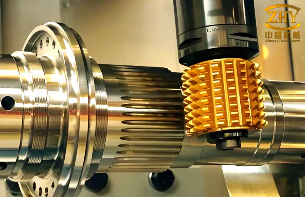
After the simulation, I performed actual cutting experiments on a five-axis vertical machining center. The blank material was a tough yellow resin, which is suitable for rapid verification of the tool path and the tooth form. The cutter was a 35° dovetail milling arbor with three indexable inserts. The verified NC code was loaded into the controller, and the pinion and gear were machined. The machined pinion and gear showed complete tooth profiles with smooth flanks and no visible chatter marks. The gear machining process was stable, and the cutter remained clear of the fixture throughout the operation.
I then evaluated the contact pattern on a computer-controlled bevel gear rolling tester. Red lead paste was applied to the working flanks of the pinion and the gear. The pair was rolled under a light load, and the contact imprint was recorded. The contact trace on the pinion concave flank appeared near the pitch line, and the contact zone was located in the middle of the tooth surface. The actual contact imprint agreed with the contact analysis of the modified tooth surface. No edge contact was observed, and the contact area was well separated from the tooth boundaries. This result confirms that the preset transmission error modification and the proposed digital generating gear machining method work together as intended.
Discussion. The proposed design and gear machining framework differs from classical bevel gear practice in several ways. First, the contact path is prescribed as a spatial curve rather than being indirectly inherited from a generating surface. Second, the pure-rolling condition is imposed directly at the kinematic level, which eliminates the sliding velocity at the contact point. Third, the tooth surface is generated from a section curve in the normal plane of the contact trace, so the local contact ellipse and the curvature interference can be controlled analytically. Fourth, the transmission error is preseeded as a parabola, which converts the theoretically zero-error pure-rolling pair into a pair with controlled sensitivity to assembly error. Fifth, the gear machining path is derived from the same conjugate geometry, so the design and manufacturing models are consistent.
The numerical experiments show that the second-order contact analysis is reliable. The relative normal curvature and relative geodesic torsion determine the contact ellipse orientation and size. In the example, the contact ellipse is oriented favorably with respect to the contact trace, and the curvature interference condition is satisfied. The modification shifts the contact zone toward the middle of the tooth surface and prevents the concentration of stress at the edges. The finite element contact analysis confirms that the actual transmission error curve follows the preset parabola and that the meshing transition points do not produce excessive angular acceleration.
The gear machining experiments show that a general disc milling cutter can produce the modified tooth surface without a dedicated bevel gear generator. The cutter location calculation is based on tangency between the cutter profile and the tooth surface. The use of the side edge for the concave flank and the bottom edge for the convex flank prevents interference. The tool path is generated by discretizing the tooth surface into layers and by moving the cutter along the instantaneous contact trace within each layer. The intermediate cutter locations are obtained by interpolation between the boundary locations. The simulated and measured errors are below a few micrometers, which is remarkable for a flexible machining process.
Several limitations remain. The current study does not include a full dynamic model of the gear pair, and the elastic deformation of the tooth body is considered only through finite element contact analysis. The thermal effect during high-speed gear machining is not explicitly modeled. The experiments were performed on resin blanks, so the behavior of hardened steel and the tool wear rate still need to be investigated. The cutter location algorithm assumes a rigid cutter and a rigid machine tool; in practice, geometric errors of the machine axes and tool runout will affect the final tooth surface. Future work should therefore include a machine tool error model, a thermal compensation strategy, and a more detailed dynamic analysis of the pure-rolling contact pair.
Conclusion. I have developed a complete design and gear machining methodology for pure-rolling contact bevel gears. The main findings are as follows. First, the continuous pure-rolling condition forces the contact trace to lie on the pitch cone, and it determines the relation between the contact parameter and the motion parameter. Second, the conjugate curve is unique for a prescribed normal direction along the contact trace, and the curve-to-surface extension produces an admissible tooth surface without local interference. Third, the second-order contact analysis gives explicit expressions for the relative normal curvature and relative geodesic torsion, which are used to select the section curve and to avoid curvature interference. Fourth, a parabolic transmission error can be preseeded by rotating the contact trace, and the resulting modification reduces the sensitivity to assembly error while keeping the contact zone away from the edges. Fifth, the digital generating gear machining method with a disc milling cutter can machine the modified pinion and the theoretical gear with errors below \(0.002\) mm. Sixth, the rolling test shows that the contact imprint is located near the pitch line and in the middle of the tooth surface, which agrees with the design intent. The proposed method therefore offers a practical route for the design and gear machining of high-performance bevel gears with pure rolling contact.