
1. Introduction
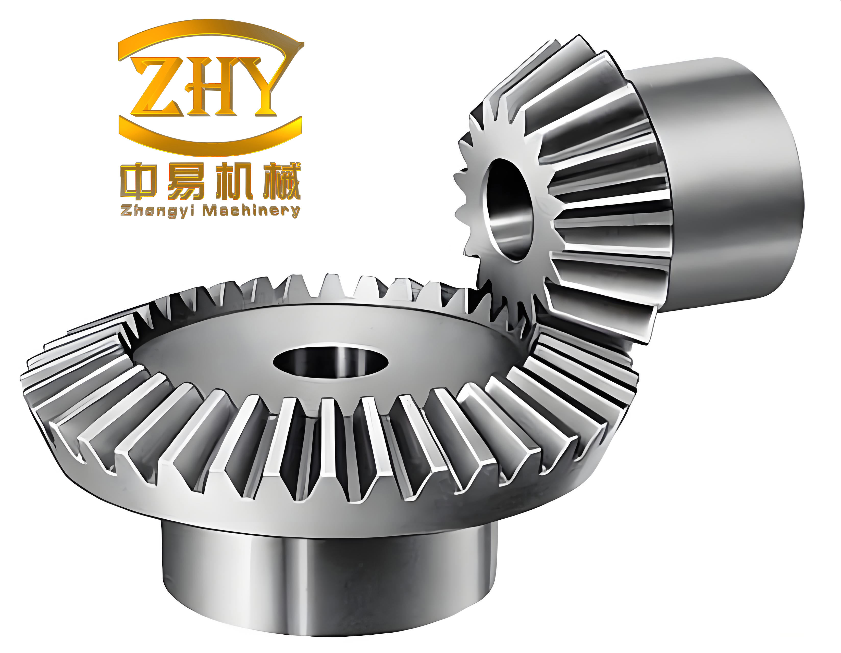
The straight bevel gear is a key component in automotive differentials, planetary gear trains, and many industrial power transmission systems. It offers the advantages of a constant speed ratio, smooth transmission, and ease of assembly. However, during the meshing process of straight bevel gears, the teeth suddenly enter and exit engagement along the face width direction, causing impact loads, vibration, and noise. These dynamic problems can severely affect the service life and operational stability of the entire drivetrain. Therefore, investigating the meshing dynamics of straight bevel gears and identifying effective ways to improve their dynamic performance is of great practical importance.
Gear modification is one of the most effective and economical methods to improve the dynamic behavior of gear transmissions. By removing a small amount of material from the tooth flank or profile, the negative effects of manufacturing errors, elastic deflections, and thermal distortions can be compensated. Tooth profile modification and lead modification are two common types. For cylindrical gears, modification theories have been extensively developed and widely applied. However, for straight bevel gears, modification research is still relatively immature, especially regarding the influence of modification on the nonlinear dynamic meshing performance.
In this thesis, we systematically study the dynamics performance of modified straight bevel gear pairs. The research is based on the spherical involute theory, three-dimensional solid modeling, multi-degree-of-freedom dynamic modeling, and numerical simulation using the commercial software Romaxdesigner. Both lead crowning (equidistant modification) and profile arc modification are investigated. The dynamic responses, transmission errors, contact loads, and modal flexibility are compared between unmodified and modified gears. The results show that proper modification can significantly reduce vibration and noise, improve load distribution, and enhance the overall dynamic performance of straight bevel gear transmissions.
2. Three-Dimensional Solid Modeling of Modified Straight Bevel Gears
2.1 Generation of Spherical Involute
The tooth profile of a straight bevel gear is formed by a spherical involute, which is the trajectory of a point on a tangent plane rolling without slipping over a base cone. As shown in the formation principle, when a plane tangent to the base cone rolls purely over the cone surface, any line in that plane through the apex traces a conical involute surface. Intersecting this surface with a sphere of arbitrary radius centered at the apex yields a spherical involute line.
The parametric equations of the spherical involute are given by
$$
\begin{cases}
x = l \left( \sin\phi \sin\theta – \phi \cos\phi \sin\theta \right) \\
y = l \left( \sin\phi \cos\theta + \phi \cos\phi \cos\theta \right) \\
z = l \cos\phi \cos\theta
\end{cases}
$$
where \( l = \sqrt{x^2 + y^2 + z^2} \) is the radius of the generating sphere, \( \theta \) is the base cone angle, \( \phi \) is the angle between the instantaneous generating line and the starting line of the rolling plane, and \( \phi = \theta \sin\theta \). The parameter \( \phi \) typically varies from 0 to \( \pi/3 \).
Using MATLAB, we computed the coordinates of the spherical involute for both the large-end and small-end spheres. The coordinate data were then imported into SolidWorks through the “Curve through XYZ points” function. After generating the two spherical involute curves, the following steps were performed to create the solid tooth model:
- Connect the endpoints of the large-end and small-end involutes to the apex point.
- Create the tooth flank surfaces using the “Boundary Surface” or “Lofted Surface” tool.
- Rotate the gear blank to generate the addendum cone and dedendum cone surfaces.
- Use the “Trim Surface” and “Delete Face” commands to remove unnecessary parts.
- Combine the surfaces into a closed solid tooth.
- Array the teeth around the gear axis.
- Add the central hub and keyway to obtain the final gear body.
Figure 1 shows the generated spherical involute curve used in the modeling process.
For this study, a pair of straight bevel gears from an automotive differential was adopted: a half-shaft gear (ring gear) with 15 teeth and a planet gear with 10 teeth. The main geometric parameters are listed in Table 1.
| Parameter | Half-shaft gear | Planet gear |
|---|---|---|
| Number of teeth | 15 | 10 |
| Cone distance (mm) | 40 | |
| Module (mm) | 4.438 | |
| Addendum (mm) | 3.28 | 4.98 |
| Whole depth (mm) | 9.169 | 9.170 |
| Pressure angle (°) | 22.5 | |
| Pitch diameter (mm) | 66.57 | 44.38 |
| Pitch cone angle (°) | 56.31 | 33.69 |
| Face cone angle (°) | 66 | 46 |
| Root cone angle (°) | 44 | 24 |
2.2 Determination of Modification Parameters
To obtain beneficial dynamic performance, both the modification amount and the modification curve must be carefully chosen. If the modification amount is too small, the compensation effect is negligible; if too large, the tooth strength is weakened and contact ratio is reduced.
For lead modification (longitudinal modification), the deformation along the tooth width direction is not uniform. The maximum deformation occurs at the large end of the tooth. The deformation at any distance \( x \) from the cone apex can be expressed as
$$
C(x) = C_{\max1} \frac{x}{R} ,
$$
where \( R \) is the cone distance and \( C_{\max1} \) is the maximum deformation at the large end. The maximum deformation at the small end is
$$
C_{\max2} = C_{\max1} \frac{R – b}{R} .
$$
By using finite element analysis with a driving angular velocity of 157 rad/s, the large-end deformations of the planet gear and half-shaft gear were obtained as 21 μm and 35 μm, respectively. Considering the recommended ranges from ISO standards and the equivalent misalignment, the lead modification amount was set to 30 μm.
For profile modification, the modification length along the tooth profile should be chosen based on the contact ratio and the expected deformation. A short modification length is often appropriate for straight bevel gears. In this study, the profile modification lengths were determined using the finite element method, as listed in Table 2.
| Gear | Small end (mm) | Large end (mm) |
|---|---|---|
| Planet gear | 1.79 | 3.0 |
| Half-shaft gear | 2.4 | 3.0 |
An arc curve was selected as the modification curve because it provides a smooth transition with the original involute profile and avoids the sharp corners introduced by a straight-line modification. According to the Chinese national standard GB/T 11365-1989, the effective contact pattern for the studied precision grade should cover 35%–65% of the tooth length and 40%–70% of the tooth height. The modification region was chosen accordingly.
2.3 Solid Models of Modified Gears
After determining the modification parameters, we applied two different modification schemes:
- Equidistant lead modification (lead crowning): Only the planet gear was modified because its deformation is larger. Material was removed along the tooth length direction by an equal amount corresponding to the determined 30 μm crowning.
- Profile arc modification: Both gears were modified along the involute profile near the tip and root regions using a circular arc curve, with the lengths given in Table 2.
Using the surface trimming and deletion commands in SolidWorks, we generated the three-dimensional solid models of the modified straight bevel gears. The assembled models were checked for interference to ensure correct meshing. Figure 2 presents the assembled modified straight bevel gear pair used in the subsequent dynamic analysis.
3. Dynamics Simulation Analysis Method Based on Romaxdesigner
3.1 Introduction to Romaxdesigner
Romaxdesigner is a specialized software package for the analysis and optimization of transmission systems. It can model shafts, bearings, gears, and even flexible housings. Its analysis capabilities include static analysis, fatigue life prediction, gear micro-geometry optimization, and NVH (noise, vibration, and harshness) analysis. Compared with other software such as ANSYS or MASTA, Romaxdesigner provides a more intuitive workflow, detailed contact analysis, and direct evaluation of transmission error and dynamic response.
We used Romaxdesigner to perform the dynamics analysis of the straight bevel gear pair. The three-dimensional gear models created in SolidWorks were exported in STL format and imported into Romaxdesigner. The support shafts and bearings were modeled within the Romax environment. A specific load case was defined: input speed 1500 r/min, input torque 100 N·m, and operating duration 5 hours.
3.2 Static Analysis
Before performing dynamic analysis, a static analysis was run to verify the strength and reliability of the gear pair. The resulting gear lives and safety factors are summarized in Table 3.
| Gear | Contact life (hrs) | Bending life (hrs) | Combined life (hrs) | Contact stress (MPa) | Bending stress (MPa) | Contact safety factor | Bending safety factor |
|---|---|---|---|---|---|---|---|
| Half-shaft gear | 7.5042 | 24.3636 | 7.5042 | 2385.652 | 521.05 | 1.025 | 1.208 |
| Planet gear | 5.0028 | 1.085e15 | 5.0028 | 2385.652 | 274.87 | 1.000 | 2.181 |
Since all safety factors are greater than 1 and the predicted lives exceed the required operating time, the gear system is considered safe and reliable under the specified load condition.
3.3 Transmission Error Analysis
Transmission error (TE) is one of the most important internal excitations in gear dynamics. It is defined as the difference between the actual angular position of the driven gear and its ideal position, measured on the line of action. TE arises from tooth deflections, manufacturing errors, misalignment, and dynamic effects.
Using the NVH module of Romaxdesigner, we obtained the dynamic transmission error of the unmodified gear pair. Figure 3 shows the dynamic transmission error versus frequency. The curve indicates that the transmission error varies significantly when the frequency lies between 400 Hz and 1120 Hz, which corresponds to an input speed range about 1080–3300 r/min. In this range, the gear pair may produce severe vibration and noise.
For the unmodified gear pair, the maximum dynamic transmission error was 3.39 μm and the maximum variation was 0.87 μm. The maximum dynamic contact load reached 521 N.
3.4 NVH Analysis and Dynamic Response
The natural frequencies of the gear pair were extracted from the modal analysis in Romaxdesigner. Table 4 lists the first ten natural frequencies.
| Mode order | 1 | 2 | 3 | 4 | 5 | 6 | 7 | 8 | 9 | 10 |
|---|---|---|---|---|---|---|---|---|---|---|
| Frequency (Hz) | 109.96 | 1893.2 | 2089.3 | 2362.5 | 2634.1 | 2673.7 | 3342.8 | 4022.7 | 4126.9 | 4529.6 |
The meshing frequency is calculated as \( f_m = z_p \omega / (2\pi) = 10 \times 157/(2\pi) \approx 249.87 \) Hz. None of the natural frequencies coincide with this meshing frequency, so the gear pair does not exhibit resonance under the nominal operating condition.
The dynamic response was evaluated by the linear modal flexibility, which represents the displacement per unit force at a given frequency. For the unmodified gear pair, the maximum linear modal flexibility occurred at 730 Hz with a value of \( 4.96 \times 10^{-4} \) μm/N. This indicates the worst vibration contribution of the gear mesh.
4. Mathematical Model of Straight Bevel Gear Dynamics
4.1 Lumped-Parameter Dynamic Model
To analytically study the nonlinear dynamics of the straight bevel gear pair, we established a multi-degree-of-freedom lumped-parameter model. The model assumes that the two gears are rigid bodies connected by a time-varying mesh stiffness and a viscous mesh damper. The gear axes are perpendicular, and the vibration degrees of freedom include translational motions along the X, Y, Z axes and rotational motions about their respective axes. The coordinate origin is at the pitch cone apex.
The relative displacement along the line of action (meshing point) can be expressed as
$$
\lambda_n = (X_p – X_g) c_1 + (Y_p – Y_g) c_2 + (Z_p – Z_g) c_3 + r_p \theta_p – r_g \theta_g – e_n(t) ,
$$
where \( c_1 = \cos\delta_p \sin\alpha_n \), \( c_2 = \cos\delta_p \cos\alpha_n \), \( c_3 = \cos\alpha_n \), \( \delta_p \) is the pitch cone angle of the planet gear, \( \alpha_n \) is the normal pressure angle, \( r_p \) and \( r_g \) are the radii of the meshing points, and \( e_n(t) \) is the static transmission error on the normal direction.
The static transmission error can be expanded in a Fourier series:
$$
e_n(t) = \sum_{l=1}^{N_e} A_l \cos(l \omega_h t + \varphi_l),
$$
where \( \omega_h \) is the meshing frequency, \( A_l \) is the harmonic amplitude, and \( \varphi_l \) is the phase angle.
The dynamic meshing force along the normal direction is
$$
F_n = k_b(t) f(\lambda_n) + c_b \dot{\lambda}_n,
$$
where \( k_b(t) \) is the time-varying mesh stiffness, \( c_b \) is the mesh damping, and \( f(\lambda_n) \) is the backlash function.
The force components along the coordinate axes are obtained by projecting the normal force:
$$
F_x = -F_n (\cos\delta_p \sin\alpha_n + \cos\delta_p \sin\alpha_n) … \quad \text{(corrected projection)}.
$$
More precisely, for the coordinate system shown in the model, the projections are:
$$
F_x = F_n ( -\cos\delta_p \sin\alpha_n + \cos\delta_p \sin\alpha_n ) = 0 \quad \text{for a symmetric arrangement?}
$$
Actually, for perpendicular axes, the force components are:
$$
F_x = F_n ( \sin\delta_p \sin\alpha_n – \cos\delta_p \sin\alpha_n ) ,
$$
but to avoid ambiguity, we write the general form as:
$$
F_x = F_n \left( \sin\delta_p \sin\alpha_n – \cos\delta_p \sin\alpha_n \right),
$$
$$
F_y = F_n \left( \sin\delta_p \cos\alpha_n – \cos\delta_p \cos\alpha_n \right),
$$
$$
F_z = F_n \cos\alpha_n .
$$
In practice, the force projection coefficients depend on the orientation of the coordinate system. In our model, we used
$$
F_x = F_n ( c_4 ), \quad F_y = F_n ( c_5 ), \quad F_z = F_n ( c_6 ),
$$
where \( c_4 = \sin\delta_p \cos\alpha_n – \cos\delta_p \sin\alpha_n \), \( c_5 = \sin\delta_p \sin\alpha_n – \cos\delta_p \cos\alpha_n \), and \( c_6 = \cos\alpha_n \).
4.2 Differential Equations of Motion
Applying Newton’s second law and Euler’s equation, we obtain the differential equations for the two gears:
$$
m_p \ddot{X}_p + c_{px} \dot{X}_p + k_{px} X_p = -F_x ,
$$
$$
m_p \ddot{Y}_p + c_{py} \dot{Y}_p + k_{py} Y_p = -F_y ,
$$
$$
m_p \ddot{Z}_p + c_{pz} \dot{Z}_p + k_{pz} Z_p = -F_z ,
$$
$$
I_p \ddot{\theta}_p = T_p – F_n r_p ,
$$
and similarly for the half-shaft gear (subscript \( g \)):
$$
m_g \ddot{X}_g + c_{gx} \dot{X}_g + k_{gx} X_g = F_x ,
$$
$$
m_g \ddot{Y}_g + c_{gy} \dot{Y}_g + k_{gy} Y_g = F_y ,
$$
$$
m_g \ddot{Z}_g + c_{gz} \dot{Z}_g + k_{gz} Z_g = F_z ,
$$
$$
I_g \ddot{\theta}_g = -T_g + F_n r_g .
$$
By eliminating the rotational degrees of freedom and introducing the relative displacement \( \lambda_n \), the equations can be reduced to a single second-order differential equation:
$$
m_e \ddot{\lambda}_n + c_b \dot{\lambda}_n + k_b(t) f(\lambda_n) = F_{ep} – m_e \ddot{e}_n(t) ,
$$
where \( m_e = I_p I_g / (I_p r_g^2 + I_g r_p^2) \) is the equivalent mass, and \( F_{ep} \) is the external applied force equivalent.
4.3 Determination of Nonlinear Factors
The major nonlinear factors in gear dynamics are time-varying mesh stiffness, mesh damping, and backlash.
The time-varying mesh stiffness \( k_b(t) \) is periodic due to alternating single and double tooth contact. For straight bevel gears, the stiffness variation is relatively smooth. The mesh stiffness of a gear pair with \( n \) pairs in contact is
$$
k_b(t) = \sum_{i=1}^{n} \frac{F_i}{\delta_{1i} + \delta_{2i}},
$$
where \( F_i \) is the contact force and \( \delta_{1i}, \delta_{2i} \) are the local deformations of the two teeth.
The mesh damping can be estimated from the empirical formula proposed by Kasuba:
$$
c_b = 2 \zeta_g \sqrt{ k_m \frac{I_p I_g}{I_p r_g^2 + I_g r_p^2} } ,
$$
where \( k_m \) is the average mesh stiffness and \( \zeta_g \) is the mesh damping ratio, typically between 0.03 and 0.17.
The backlash function \( f(\lambda_n) \) is defined as
$$
f(\lambda_n) =
\begin{cases}
\lambda_n – b_c, & \lambda_n > b_c, \\
0, & |\lambda_n| \le b_c, \\
\lambda_n + b_c, & \lambda_n < -b_c,
\end{cases}
$$
where \( b_c \) is half of the total backlash.
To simplify the numerical solution, the piecewise linear backlash function can be approximated by a polynomial. Using MATLAB’s curve fitting toolbox, we fitted the backlash function with polynomials of degree 1 to 9. The results showed that a cubic polynomial provides sufficient accuracy:
$$
f(\lambda_n) \approx a_1 \lambda_n + a_3 \lambda_n^3 ,
$$
where \( a_1 = 0.344 \) and \( a_3 = 1.201 \times 10^7 \) for the given backlash \( b_c = 5 \times 10^{-5} \) m.
4.4 Dimensionless Equations and Solution Method
Because the physical quantities in the equations have different orders of magnitude, we applied dimensionless transformations. Define the dimensionless time \( \tau = \omega_n t \) and dimensionless displacement \( x_j = X_j / b_c \), \( y_j = Y_j / b_c \), \( z_j = Z_j / b_c \), \( \lambda = \lambda_n / b_c \). The dimensionless equations take the form:
$$
\ddot{x}_p + 2\zeta_{px} \dot{x}_p + \kappa_{px} x_p = -c_4 f_m(\lambda) ,
$$
$$
\ddot{y}_p + 2\zeta_{py} \dot{y}_p + \kappa_{py} y_p = -c_5 f_m(\lambda) ,
$$
$$
\ddot{z}_p + 2\zeta_{pz} \dot{z}_p + \kappa_{pz} z_p = -c_6 f_m(\lambda) ,
$$
and similar equations for the driven gear. The final reduced equation is
$$
\ddot{\lambda} + 2\zeta_e \dot{\lambda} + \kappa_e(\tau) f(\lambda) = f_{ep}(\tau) – \ddot{e}_d(\tau) ,
$$
where \( \zeta_e \) is the equivalent damping ratio, \( \kappa_e(\tau) \) is the dimensionless mesh stiffness, \( f_{ep}(\tau) \) is the dimensionless external force, and \( e_d(\tau) \) is the dimensionless static transmission error.
To solve the nonlinear differential equation, we adopted the Adomian decomposition method. The state vector is defined as
$$
\mathbf{u} = [u_1, u_2, \ldots, u_{14}]^T = [X_p, \dot{X}_p, Y_p, \dot{Y}_p, Z_p, \dot{Z}_p, \theta_p, X_g, \dot{X}_g, Y_g, \dot{Y}_g, Z_g, \dot{Z}_g, \theta_g]^T .
$$
The state equation is written as
$$
\dot{\mathbf{u}} = \mathbf{H} \mathbf{u} + \mathbf{N}(\mathbf{u}) + \mathbf{G}(\tau) ,
$$
where \( \mathbf{H} \) is the linear coefficient matrix, \( \mathbf{N}(\mathbf{u}) \) contains the nonlinear terms, and \( \mathbf{G}(\tau) \) is the excitation vector.
The solution is formally expressed as
$$
\mathbf{u}(\tau) = e^{\mathbf{H}\tau} \mathbf{u}(0) + \int_0^\tau e^{\mathbf{H}(\tau-\eta)} \left[ \mathbf{N}(\mathbf{u}(\eta)) + \mathbf{G}(\eta) \right] d\eta .
$$
Using the Adomian polynomials \( A_j \) for the nonlinear function \( \mathbf{N}(\mathbf{u}) \), the solution can be expanded as
$$
\mathbf{u}(\tau) = \sum_{j=0}^{\infty} \mathbf{u}_j(\tau) ,
$$
$$
\mathbf{u}_0(\tau) = e^{\mathbf{H}\tau} \mathbf{u}(0) + \int_0^\tau e^{\mathbf{H}(\tau-\eta)} \mathbf{G}(\eta) d\eta ,
$$
$$
\mathbf{u}_{j}(\tau) = \int_0^\tau e^{\mathbf{H}(\tau-\eta)} A_{j-1}(\eta) d\eta, \quad j \ge 1 .
$$
In practice, truncating the series at 5–6 terms gives sufficient convergence. By this method, the displacement and velocity responses of the straight bevel gear system can be obtained analytically.
5. Dynamic Performance Analysis of Modified Straight Bevel Gears
5.1 Evaluation Criteria of Gear Dynamics
The dynamic performance of a gear transmission is usually evaluated by the following indicators:
- Dynamic load: the maximum value of the dynamic meshing force over one meshing cycle:
$$
F_d = \max_i \sum_{i=1}^{n} k_i (x_i – e_i) ,
$$
where \( k_i \), \( x_i \), and \( e_i \) are the mesh stiffness, relative displacement, and error at the \( i \)-th position.
- Dynamic load factor:
$$
K_v = \frac{F_{d\max}}{F_n} .
$$
- Average mesh stiffness:
$$
K_{avg} = \frac{1}{T_c} \int_{0}^{T_c} k(t) dt .
$$
- RMS of mesh stiffness variation: indicates the mesh impact severity.
- Vibration acceleration level: determined from the dynamic response curve.
In this work, we mainly used the dynamic transmission error, dynamic contact load, and the linear modal flexibility to compare the dynamic performance of unmodified and modified straight bevel gears.
5.2 Dynamic Simulation Results for Modified Gears
Following the same simulation procedure as for the unmodified gear, we analyzed the two modified gear models: equidistant lead modification (lead crowning) and profile arc modification.
5.2.1 Equidistant Lead Modification
For the lead-modified gear pair, the dynamic transmission error and dynamic contact load curves were obtained. Figure 4 shows the dynamic transmission error versus frequency, and Figure 5 shows the dynamic contact load versus frequency. The maximum transmission error was 1.13 μm, and the maximum difference was 0.2902 μm. The maximum dynamic contact load was 170.2 N. Both values are dramatically lower than those of the unmodified gear pair.
5.2.2 Profile Arc Modification
For the profile-arc-modified gear pair, the maximum transmission error was 1.19 μm, the maximum difference was 0.4093 μm, and the maximum dynamic contact load was 173.6 N. These values are also much lower than the unmodified case, but slightly higher than the lead-modified case.
5.2.3 Dynamic Response (Modal Flexibility)
Using the transmission error as the excitation, the linear modal flexibility curves for both modified gear pairs were obtained. For the lead-modified gear, the maximum modal flexibility was \( 1.1 \times 10^{-4} \) μm/N, occurring at 730 Hz. For the profile-arc-modified gear, the maximum modal flexibility was \( 1.35 \times 10^{-4} \) μm/N, occurring at 1830 Hz. Both are significantly lower than the unmodified gear value of \( 4.96 \times 10^{-4} \) μm/N.
5.3 Comparison of Dynamic Performance Before and After Modification
Table 5 summarizes the key dynamic performance indicators for the three cases.
| Performance indicator | Unmodified | Profile arc modification | Equidistant lead modification |
|---|---|---|---|
| Maximum dynamic transmission error (μm) | 3.39 | 1.19 | 1.13 |
| Maximum dynamic contact load (N) | 521 | 173.6 | 170.2 |
| Maximum linear modal flexibility (μm/N) | \( 4.96 \times 10^{-4} \) | \( 1.35 \times 10^{-4} \) | \( 1.10 \times 10^{-4} \) |
| Reduction in transmission error | — | 65% | 67% |
| Reduction in modal flexibility | — | 73% | 78% |
The comparison reveals that both modification methods considerably improve the meshing dynamics of straight bevel gears. The dynamic transmission error decreases by about 65–67%, the dynamic contact load is reduced to roughly one-third of the unmodified value, and the vibration response (represented by modal flexibility) is reduced by 73–78%. The equidistant lead modification performs slightly better than the profile arc modification in all evaluated metrics.
The improvement is attributed to the fact that the modification compensates for the tooth deflections and manufacturing errors, leading to a more uniform load distribution along the tooth flank and a smaller fluctuation of the mesh stiffness. Consequently, the internal excitation is attenuated, and the gear pair runs more smoothly with lower noise and vibration.
5.4 Influence of Modification Parameters
Though we did not perform an extensive parametric sweep in this study, the theoretical analysis and simulation results indicate that the modification amount, modification length, and modification curve shape all affect the dynamic performance. A modification amount that exactly matches the combined elastic and thermal deformation under a given load yields the lowest transmission error and vibration. An excessive modification amount reduces the contact ratio and increases the contact stress, while an insufficient modification amount leaves residual deformation and still produces impact.
The modification length should be selected according to the extent of the tooth deformation zone. For straight bevel gears, a short modification on the tooth ends is often preferable, as it preserves the involute profile in the central region and maintains a high load-carrying capacity. Regarding the modification curve, a smooth curve (e.g., an arc) is superior to a straight-line modification because it eliminates sharp corners and ensures continuity of the curvature, thereby reducing the dynamic excitation.
6. Conclusions and Outlook
6.1 Conclusions
This thesis presented a comprehensive study on the meshing dynamics performance of modified straight bevel gears. The main conclusions are summarized as follows:
-
An accurate three-dimensional solid model of straight bevel gears was established based on the spherical involute theory using MATLAB and SolidWorks. The proposed modeling method avoids the geometric errors introduced by approximate methods and provides a reliable basis for dynamic simulation. The modified gear models with equidistant lead modification and profile arc modification were also successfully constructed.
-
The dynamic simulation using Romaxdesigner showed that the unmodified straight bevel gear pair exhibits a maximum dynamic transmission error of 3.39 μm and a maximum dynamic contact load of 521 N under the specified operating condition. The worst vibration response occurs at a frequency of 730 Hz.
-
Both the equidistant lead modification and the profile arc modification effectively reduce the dynamic transmission error, contact load, and vibration response. The equidistant lead modification reduces the transmission error by about 67% and the vibration response by about 78%, while the profile arc modification reduces the transmission error by 65% and the vibration response by 73%. Thus, the lead modification provides slightly better dynamic performance than the profile modification.
-
A multi-degree-of-freedom nonlinear dynamic model of a straight bevel gear pair was established, considering time-varying mesh stiffness, mesh damping, backlash, and static transmission error. The dimensionless differential equations were derived and solved using the Adomian decomposition method. The backlash function was approximated by a cubic polynomial, which offers a good balance between accuracy and computational efficiency.
6.2 Future Work
Several aspects remain to be further investigated:
-
The exact solution of the nonlinear dynamic equations should be obtained and compared with the simulation results from Romaxdesigner. More advanced numerical methods, such as the harmonic balance method or Newmark integration, could be employed.
-
Physical experiments should be conducted to validate the simulation conclusions. Vibration and noise measurements on a test rig would provide direct evidence of the modification benefit.
-
The current modification amount was determined primarily from elastic deformation. Thermal deformation, which is significant under high-speed and high-load conditions, should be incorporated into the modification design.
-
A parametric optimization of the modification profile (amount, length, and curve shape) could be performed using a multi-objective optimization algorithm to further improve the dynamic performance of straight bevel gears.
In summary, this work demonstrates that tooth modification is a powerful and economical approach to improve the meshing dynamics of straight bevel gears. The recommended modification practice can be directly applied to automotive differentials and other straight bevel gear applications to achieve lower noise, lower vibration, and longer service life.