
In my work on high-precision manufacturing of spiral bevel gear sets, I treat tooth flank machining error as a measurable, parameter-driven deviation between the actual ground surface and the theoretical design surface. My objective is to reduce this deviation by correcting the machine settings that govern the duplex helical generation process. I begin with a coordinate-based model of the spiral bevel gear tooth flank, then build an error control model, evaluate the sensitivity of each machine setting, and solve the compensation problem with an improved Levenberg-Marquardt algorithm. The result is a practical machine-setting correction method that can be applied to real spiral bevel gear production without changing the basic cutter geometry or the fundamental cutting cycle.
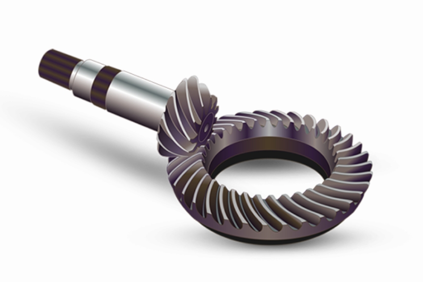
1. Introduction
Spiral bevel gear pairs are widely used in aerospace drivetrains, automotive axles, marine transmissions, and other high-load motion systems. Their teeth are curved, their contact pattern is sensitive to small geometric changes, and their manufacturing accuracy directly affects vibration, noise, fatigue life, and transmission efficiency. In actual production, unavoidable errors arise from machine tool geometry, thermal drift, servo following error, cutter wear, fixture compliance, and workpiece mounting. These errors change the relative position and relative motion between the cutter and the workpiece, and therefore they change the final spiral bevel gear tooth flank.
I focus on the duplex helical method because it is one of the most important generation methods for spiral bevel gear teeth. In this method, the cutter head represents a virtual generating gear. The cutter rotates, the workpiece rotates in a timed relationship, and the tool is fed along a controlled path. The resulting spiral bevel gear tooth flank is a conjugate envelope of the cutter blade family. Because the process is nonlinear and strongly coupled, a direct trial-and-error correction of machine settings is expensive and unreliable. I therefore formulate the correction as a numerical optimization problem driven by measured tooth flank error.
The central idea of my method is simple: if the actual spiral bevel gear tooth flank deviates from the theoretical flank by a normal error distribution, then a small correction of selected machine settings can produce an opposite normal displacement. I use coordinate homogeneous transformation and meshing theory to relate machine settings to the generated spiral bevel gear surface. I then compute the normal distance between measured and theoretical points. The sensitivity of each machine setting is evaluated over the whole tooth flank, and the most influential settings are selected as optimization variables. Finally, an improved Levenberg-Marquardt algorithm solves for the correction values. The method is validated on a real spiral bevel gear pair produced by duplex helical grinding.
2. Nomenclature and Basic Definitions
| Symbol | Meaning |
|---|---|
| \(\xi\) | Vector of duplex helical machine settings |
| \(\phi\) | Generating motion parameter |
| \(u\) | Cutter blade height parameter |
| \(\theta\) | Cutter blade rotational parameter |
| \(\mathbf{r}(u,\theta)\) | Digital representation of the cutter blade surface |
| \(\mathbf{M}_{bc}\) | Homogeneous transformation matrix from cutter to workpiece |
| \(\mathbf{F}(\xi)\) | Family of surfaces generated by the cutter |
| \(\mathbf{n}\) | Unit normal vector on the generated surface |
| \(\mathbf{v}\) | Relative velocity between cutter and workpiece |
| \(\mathbf{P}_{CMM,i}\) | Measured point on the actual spiral bevel gear tooth flank |
| \(h_i\) | Normal error at the \(i\)-th measured point |
| \(\mathbf{J}\) | Jacobian or sensitivity matrix |
| \(\Delta\xi\) | Machine-setting correction vector |
| \(\varepsilon_j\) | Comprehensive sensitivity coefficient of the \(j\)-th setting |
| \(\lambda_k\) | Levenberg-Marquardt damping parameter at iteration \(k\) |
| \(\mu\) | Damping adjustment factor |
| \(h_{\max}\) | Maximum absolute residual error |
| \(h_{goal}\) | Target maximum absolute error |
The machine-setting vector in my model is written as
$$
\xi = [q,\ S_R,\ E_M,\ X_D,\ X_B,\ \gamma_m,\ R_a,\ m_c,\ d_q,\ \chi_{HL}]
$$
where \(q\) is the angular cutter position, \(S_R\) is the radial cutter position, \(E_M\) is the vertical offset, \(X_D\) is the horizontal offset, \(X_B\) is the bed position, \(\gamma_m\) is the mounting angle, \(R_a\) is the cutter rotation angle, \(m_c\) is the roll ratio, \(d_q\) is the cutter tilt angle, and \(\chi_{HL}\) is the spiral correction coefficient. Each of these settings influences the final spiral bevel gear tooth flank in a different way.
3. Mathematical Model of Spiral Bevel Gear Duplex Helical Generation
The first step in my compensation method is to build an accurate mapping from machine settings to the spiral bevel gear tooth flank. I use homogeneous coordinate transformation because it allows the cutter, the workpiece, and all intermediate frames to be expressed in a unified algebraic form. The cutter blade is modeled as a surface parameterized by \(u\) and \(\theta\). The family of surfaces generated during the cutting motion is
$$
\mathbf{F}(\xi) = \mathbf{M}_{bc}(q,S_R,E_M,X_B,\gamma_m,R_a,m_c,d_q,\chi_{HL};\phi)\,\mathbf{r}(u,\theta)
$$
For a fixed machine-setting vector \(\xi\), the generated spiral bevel gear tooth flank is the envelope of this family. According to meshing theory, the envelope condition is that the relative velocity between the cutter and the workpiece is perpendicular to the surface normal. Therefore I write
$$
\begin{cases}
\mathbf{F}(\xi) = \mathbf{M}_{bc}(\xi,\phi)\,\mathbf{r}(u,\theta) \\
f(\xi) = \mathbf{n}\cdot\mathbf{v}
= \left(\dfrac{\partial \mathbf{F}(\xi)}{\partial u}
\times \dfrac{\partial \mathbf{F}(\xi)}{\partial \theta}\right)
\cdot \dfrac{\partial \mathbf{F}(\xi)}{\partial \phi} = 0
\end{cases}
$$
The first equation describes the geometric position of the cutter surface after transformation. The second equation is the meshing equation. Together they define the spiral bevel gear tooth flank implicitly. For numerical computation, I discretize the tooth flank into a grid along the tooth height and tooth width directions. At each grid point, I solve the meshing equation and obtain the corresponding theoretical surface point and normal vector.
I write the theoretical surface point and normal vector at the \(i\)-th grid point as
$$
\mathbf{r}_i = \mathbf{r}((u,\theta,\phi)_i,\xi), \qquad
\mathbf{n}_i = \mathbf{n}((u,\theta,\phi)_i,\xi)
$$
In practice, I use a uniform grid because it makes the sensitivity analysis and error comparison stable. The grid covers the working tooth flank and, when needed, the root fillet region. The theoretical spiral bevel gear surface is then represented as a set of discrete points \(\mathbf{r}_1,\mathbf{r}_2,\ldots,\mathbf{r}_m\).
4. Tooth Flank Measurement and Error Control Model
After the spiral bevel gear is machined, I measure the actual tooth flank with a precision measuring instrument. The measured points are denoted by \(\mathbf{P}_{CMM,i}\). Because the measured points do not lie exactly on the theoretical surface, I compute the normal distance between each measured point and the theoretical spiral bevel gear surface. This normal distance is the machining error. For the \(i\)-th point, I define
$$
(\mathbf{P}_{CMM,i} – \mathbf{r}((u,\theta,\phi)_i,\xi))\cdot
\mathbf{n}((u,\theta,\phi)_i,\xi) = h_i
$$
Here, \(h_i\) is positive when the actual surface lies outside the theoretical surface along the normal direction, and negative when it lies inside. The complete error vector is
$$
\mathbf{h} = [h_1,\ h_2,\ \ldots,\ h_m]^T
$$
In engineering production, I usually require
$$
|h_i| \le 0.005\ \text{mm}
$$
for the working region of the spiral bevel gear tooth flank. This tolerance is not arbitrary. It reflects the need for stable contact patterns, low transmission error, and acceptable dynamic behavior. When the maximum absolute error exceeds this limit, the spiral bevel gear pair may still rotate, but its contact pattern and load distribution will be less predictable.
To make the error model useful for compensation, I express the actual tooth flank as a perturbation of the theoretical surface. If the machine settings change from \(\xi\) to \(\xi_e = \xi + \Delta\xi\), the actual generated surface can be written as
$$
\mathbf{r}_e(u,\theta,\phi,\xi_e) =
\mathbf{M}(\xi_e;\phi)\,\mathbf{r}(u,\theta)
$$
with the meshing condition
$$
\mathbf{n}\cdot\mathbf{v} = 0
$$
Therefore, the error vector is a nonlinear function of the machine-setting correction \(\Delta\xi\). My goal is to find a correction vector that minimizes the normal error over the measured spiral bevel gear tooth flank.
5. Sensitivity Analysis of Machine Settings
Not every machine setting has the same influence on the spiral bevel gear tooth flank. Some settings produce a global shift of the contact pattern, while others change the local curvature or the spiral angle. If I include all settings as optimization variables, the problem becomes ill-conditioned and the convergence rate drops. Therefore I perform a sensitivity analysis before optimization.
The sensitivity of the normal error with respect to a machine setting is the derivative of the error with respect to that setting. From the error definition, I obtain
$$
\dfrac{dh(\xi)}{d\xi}\bigg|_{\mathbf{P}_{CMM,i}}
=
-\dfrac{\partial \mathbf{r}_i}{\partial \xi}\cdot \mathbf{n}_i
$$
This expression is elegant because the measured point \(\mathbf{P}_{CMM,i}\) does not appear explicitly in the derivative. The sensitivity depends only on how the theoretical spiral bevel gear surface moves when the machine setting changes. For each measured point \(i\) and each machine setting \(j\), I compute the sensitivity coefficient
$$
J_{ij} = -\dfrac{\partial \mathbf{r}_i((u,\theta,\phi),\xi)}{\partial \xi_j}\cdot \mathbf{n}_i
$$
The full sensitivity matrix is
$$
\mathbf{J} =
\begin{bmatrix}
J_{11} & J_{12} & \cdots & J_{1m} \\
J_{21} & J_{22} & \cdots & J_{2m} \\
\vdots & \vdots & \ddots & \vdots \\
J_{n1} & J_{n2} & \cdots & J_{nm}
\end{bmatrix}
$$
where \(n\) is the number of measured points and \(m\) is the number of machine settings. For a small correction, the error model can be linearized as
$$
\mathbf{h} = \mathbf{J}\,\Delta\xi
$$
This linearized form is the basis of my compensation algorithm. However, because the actual relationship is nonlinear, I use it only inside an iterative Levenberg-Marquardt scheme.
To rank the settings, I compute a comprehensive sensitivity coefficient for each setting:
$$
\varepsilon_j = \dfrac{1}{n}\sum_{i=1}^{n} |J_{ij}|
$$
The larger \(\varepsilon_j\) is, the stronger the influence of the \(j\)-th machine setting on the spiral bevel gear tooth flank. I sort the settings by \(\varepsilon_j\) and select the three to five most sensitive settings as optimization variables. This step improves both efficiency and numerical stability.
| Machine setting | Role in spiral bevel gear generation | Typical sensitivity behavior |
|---|---|---|
| Radial cutter position \(S_R\) | Changes cutter center distance | Strong global effect on both flanks |
| Angular cutter position \(q\) | Rotates cutter around its axis | Asymmetric effect on concave and convex flanks |
| Mounting angle \(\gamma_m\) | Changes workpiece orientation | Strong effect on tooth height distribution |
| Roll ratio \(m_c\) | Controls generating motion ratio | Strong near tooth tip and root |
| Vertical offset \(E_M\) | Shifts workpiece vertically | Moderate local effect |
| Horizontal offset \(X_D\) | Shifts workpiece horizontally | Moderate local effect |
| Bed position \(X_B\) | Adjusts axial position | Local tooth width effect |
| Cutter tilt \(d_q\) | Changes cutter inclination | Strong curvature effect |
| Spiral correction \(\chi_{HL}\) | Modifies spiral angle distribution | Local tooth width effect |
6. Improved Levenberg-Marquardt Compensation Algorithm
Once the sensitive machine settings are selected, I solve for the correction vector \(\Delta\xi\). The compensation problem is
$$
\xi_c = \arg\min_{\xi} \dfrac{1}{2}\mathbf{h}^T(\xi)\mathbf{h}(\xi)
$$
This is a nonlinear least-squares problem. The Jacobian matrix \(\mathbf{J}\) may become ill-conditioned or nearly singular when the spiral bevel gear tooth flank is close to the target surface, or when two machine settings have similar effects. A plain Gauss-Newton method can then produce unstable corrections. Therefore I use an improved Levenberg-Marquardt algorithm.
At iteration \(k\), the correction update is
$$
\Delta\xi_{k+1} =
\Delta\xi_k –
(\mathbf{J}_k^T\mathbf{J}_k + \lambda_k\mathbf{I})^{-1}
\mathbf{J}_k^T\mathbf{F}_k
$$
where \(\lambda_k \ge 0\) is the damping parameter and \(\mathbf{F}_k\) is the residual vector at iteration \(k\). When \(\lambda_k\) is large, the update behaves like a gradient descent step and is very stable. When \(\lambda_k\) is small, the update behaves like a Gauss-Newton step and converges quickly. The key is to adjust \(\lambda_k\) according to both the actual reduction and the distance from the target error.
I define the ratio between the actual reduction and the model-predicted reduction as \(r_m\). I also monitor the maximum absolute residual \(h_{\max}\) and compare it with the target error \(h_{goal}\). The damping parameter is updated as
$$
\lambda_k = \mu \lambda_k
$$
$$
\mu =
\begin{cases}
\mu, & r_m > p_1 \\
1.5\mu, & r_m \le p_1 \ \text{or}\ h_{\max} < 2h_{goal}
\end{cases}
$$
This conditional update prevents the damping parameter from becoming too small near the optimum. When the spiral bevel gear tooth flank is already close to the target, the algorithm increases damping slightly to avoid over-correction. When the reduction ratio is poor, the algorithm also increases damping to improve stability.
I also apply three practical safeguards. First, I check whether a corrected setting exceeds its allowable range. If it does, I either clip it to the previous value or remove it from the optimization variable set. Second, I favor solutions that reduce the maximum error, because the maximum error often controls the contact pattern. Third, I set the optimization tolerance according to the initial error level and the measurement uncertainty. This avoids unnecessary iterations when the spiral bevel gear tooth flank is already within tolerance.
| Algorithm component | Traditional Levenberg-Marquardt | My improved strategy |
|---|---|---|
| Damping update | Fixed or simple reduction rule | Uses \(\mu\) and residual distance |
| Near-optimum behavior | May become unstable | Increases damping when \(h_{\max} < 2h_{goal}\) |
| Parameter bounds | Often ignored | Checks and clips or removes out-of-range settings |
| Variable selection | All settings may be used | Only high-sensitivity settings are optimized |
| Convergence focus | Mean square error | Mean square error plus maximum error |
7. Compensation Workflow
I organize the spiral bevel gear compensation method into the following steps.
- Input the initial machine settings and cutter parameters.
- Build the theoretical spiral bevel gear tooth flank model.
- Measure the actual tooth flank and compute the normal error vector \(\mathbf{h}\).
- Compute the sensitivity matrix \(\mathbf{J}\) and the comprehensive sensitivity coefficients \(\varepsilon_j\).
- Sort the machine settings and select the most sensitive three to five settings as optimization variables.
- Solve the nonlinear least-squares problem with the improved Levenberg-Marquardt algorithm.
- Check whether the corrected settings are within their allowable ranges.
- If local error is still too large, perform a local sensitivity analysis and adjust the optimization strategy.
- Output the compensated machine settings and the retained settings as a complete correction matrix.
- Validate the corrected settings by simulation and, when possible, by a real cutting or grinding test.
This workflow is iterative. In some cases, one compensation pass is enough to bring the spiral bevel gear tooth flank within tolerance. In other cases, two or three passes are needed. I can also increase the number of optimization variables in later passes if the remaining error is concentrated in a local region.
8. Application to a Spiral Bevel Gear Pair
I applied the method to a pair of spiral bevel gears produced by duplex helical grinding. The initial machine settings are listed in Table 3. The pinion and the gear have different cutter parameters and different mounting conditions. The initial measured errors exceeded the target tolerance, so compensation was necessary.
| Initial machine setting | Pinion | Gear |
|---|---|---|
| Radial cutter position \(S_R\) (mm) | 163.3098 | 163.5261 |
| Angular cutter position \(q\) (rad) | 0.8813 | 0.8694 |
| Cutter tilt \(d_q\) (rad) | 0.0603 | 0.5985 |
| Cutter rotation \(R_a\) (rad) | 0.0453 | 0.2597 |
| Vertical offset \(E_M\) (mm) | 0.12558 | 0 |
| Mounting angle \(\gamma_m\) (rad) | 0.3513 | 0.4037 |
| Horizontal offset \(X_D\) (mm) | 0.43873 | 0 |
| Bed position \(X_B\) (mm) | -3.1264 | -3.86914 |
| Roll ratio \(m_c\) | 2.5259 | 2.0754 |
| Spiral correction \(\chi_{HL}\) | 6.6848 | 0 |
I discretized the spiral bevel gear tooth flank into a \(5 \times 9\) grid to compute sensitivities. This grid size is large enough to capture the global error distribution and small enough to keep computation efficient. The sensitivity analysis showed that the radial cutter position, angular cutter position, mounting angle, and roll ratio had the largest comprehensive sensitivity coefficients. Therefore I selected these four settings as optimization variables for the pinion and the corresponding settings for the gear.
| Parameter | Comprehensive sensitivity \(\varepsilon_j\) | Rank | Selected as variable |
|---|---|---|---|
| \(S_R\) | 0.0247 | 1 | Yes |
| \(q\) | 0.0198 | 2 | Yes |
| \(\gamma_m\) | 0.0165 | 3 | Yes |
| \(m_c\) | 0.0132 | 4 | Yes |
| \(d_q\) | 0.0091 | 5 | No |
| \(E_M\) | 0.0074 | 6 | No |
| \(X_D\) | 0.0068 | 7 | No |
| \(X_B\) | 0.0055 | 8 | No |
| \(R_a\) | 0.0049 | 9 | No |
| \(\chi_{HL}\) | 0.0038 | 10 | No |
The sensitivity results also revealed an important coupling effect. For the pinion, the concave and convex flanks responded differently to the same machine setting. For example, increasing the radial cutter position tended to increase the error on the concave flank while decreasing it on the convex flank. Because the working flank of the pinion is usually the concave side, I prioritized the correction direction that reduced the concave error. For the gear, the convex flank is usually the working side, so I prioritized the convex flank in a similar way.
After two compensation passes, the corrected machine settings were obtained. Table 5 lists the adjusted values. The changes are small, which is important for practical production. Large changes can alter the contact pattern or require new cutter settings, while small changes can be absorbed by normal machine adjustment.
| Adjusted machine setting | Pinion | Gear |
|---|---|---|
| Radial cutter position \(S_R\) (mm) | 161.3222 | 161.6530 |
| Angular cutter position \(q\) (rad) | 0.8814 | 0.8692 |
| Cutter tilt \(d_q\) (rad) | 0.0603 | 0.5985 |
| Cutter rotation \(R_a\) (rad) | 0.0453 | 0.2597 |
| Vertical offset \(E_M\) (mm) | 0.12558 | 0 |
| Mounting angle \(\gamma_m\) (rad) | 0.3508 | 0.4146 |
| Horizontal offset \(X_D\) (mm) | 0.43873 | 0 |
| Bed position \(X_B\) (mm) | -3.1264 | -3.86914 |
| Roll ratio \(m_c\) | 2.5126 | 2.0803 |
| Spiral correction \(\chi_{HL}\) | 6.6848 | 0 |
9. Predicted Residual Error After Compensation
I evaluated the compensation result by predicting the residual normal error on the spiral bevel gear tooth flank. Table 6 compares the initial measurement, the first correction, and the second correction. The cumulative error and the maximum error both decreased. The first pass reduced the error but did not bring the maximum error below the target. The second pass achieved the required tolerance.
| Error measure | Flank | Initial | After pass 1 | After pass 2 |
|---|---|---|---|---|
| Cumulative error (mm) | Pinion concave | 0.3473 | 0.1705 | 0.0511 |
| Cumulative error (mm) | Pinion convex | 0.2998 | 0.1705 | 0.1181 |
| Cumulative error (mm) | Gear concave | 0.4402 | 0.1761 | 0.0763 |
| Cumulative error (mm) | Gear convex | 0.4122 | 0.2107 | 0.0485 |
| Maximum error (mm) | Pinion concave | 0.0189 | 0.0105 | 0.0031 |
| Maximum error (mm) | Pinion convex | 0.0149 | 0.0083 | 0.0047 |
| Maximum error (mm) | Gear concave | 0.0196 | 0.0130 | 0.0041 |
| Maximum error (mm) | Gear convex | 0.0178 | 0.0112 | 0.0045 |
The cumulative error on the pinion concave flank decreased by 85.29%, and the maximum error decreased by 83.70%. The pinion convex flank cumulative error decreased by 60.59%, and its maximum error decreased by 68.75%. The gear concave flank cumulative error decreased by 82.66%, and its maximum error decreased by 78.79%. The gear convex flank cumulative error decreased by 88.02%, and its maximum error decreased by 75.00%. These reductions show that the selected machine settings can control the spiral bevel gear tooth flank error effectively.
| Flank | Cumulative error reduction | Maximum error reduction |
|---|---|---|
| Pinion concave | 85.29% | 83.70% |
| Pinion convex | 60.59% | 68.75% |
| Gear concave | 82.66% | 78.79% |
| Gear convex | 88.02% | 75.00% |
10. Experimental Validation on the Spiral Bevel Gear Pair
After obtaining the corrected machine settings, I machined the spiral bevel gear pair and measured the actual tooth flanks. The measurement grid contained several rows and columns along the tooth height and tooth width. Table 8 summarizes the measured absolute errors for representative points. The maximum absolute error on the pinion concave flank was 3.5 \(\mu\)m, and the maximum absolute error on the pinion convex flank was 4.8 \(\mu\)m. The maximum absolute error on the gear concave flank was 4.7 \(\mu\)m, and the maximum absolute error on the gear convex flank was 4.3 \(\mu\)m.
| Node | Pinion concave (\(\mu\)m) | Pinion convex (\(\mu\)m) | Gear concave (\(\mu\)m) | Gear convex (\(\mu\)m) |
|---|---|---|---|---|
| A1 | 3.5 | 3.4 | 4.7 | 3.4 |
| A3 | 0.7 | 0.9 | 4.0 | 2.4 |
| A5 | 0.9 | 1.8 | 4.3 | 3.1 |
| C1 | 2.9 | 1.7 | 4.0 | 2.1 |
| C3 | 0.3 | 1.0 | 1.9 | 1.1 |
| C5 | 3.0 | 1.5 | 2.0 | 1.5 |
| E1 | 2.6 | 1.8 | 3.5 | 1.7 |
| E3 | 0.0 | 0.0 | 0.0 | 0.0 |
| E5 | 4.1 | 2.1 | 0.2 | -0.9 |
| G1 | 3.4 | 2.8 | 3.0 | 2.1 |
| G3 | 1.6 | 0.3 | 1.4 | 1.2 |
| G5 | 3.5 | 2.9 | 3.5 | 1.7 |
| I1 | 3.7 | 3.5 | 3.7 | 4.3 |
| I3 | 1.9 | 1.4 | 1.9 | 3.4 |
| I5 | 3.9 | 2.4 | 3.0 | 2.4 |
The measured errors are all below 0.005 mm. This satisfies the engineering requirement. Compared with the initial errors, the pinion concave maximum error decreased by 81.5%, and the pinion convex maximum error decreased by 67.8%. The gear concave maximum error decreased by 78.1%, and the gear convex maximum error decreased by 73.6%. The actual measurement therefore confirms the predicted improvement.
| Flank | Maximum measured error (\(\mu\)m) | Reduction relative to initial |
|---|---|---|
| Pinion concave | 3.5 | 81.5% |
| Pinion convex | 4.8 | 67.8% |
| Gear concave | 4.3 | 78.1% |
| Gear convex | 4.7 | 73.6% |
11. Discussion
Several observations emerge from my study of spiral bevel gear compensation. First, the sensitivity analysis is essential. If I optimize all machine settings simultaneously, the Jacobian matrix becomes poorly conditioned, and the correction can oscillate. By selecting the most sensitive settings, I reduce the number of variables and improve convergence. Second, the concave and convex flanks of a spiral bevel gear are coupled. A correction that improves one flank may worsen the other. My method handles this coupling by evaluating sensitivity over both flanks and by prioritizing the working flank. Third, the improved Levenberg-Marquardt algorithm provides a good balance between stability and speed. The damping parameter prevents large jumps when the solution is near the target, and the residual-based update allows fast convergence when the initial error is large.
The method is also practical. The corrected machine settings are small modifications of the original settings. They can be entered into the machine controller without redesigning the cutter or changing the basic duplex helical cycle. The required measurement is a standard tooth flank measurement, which is already available in many spiral bevel gear production lines. The computation cost is moderate because the tooth flank grid can be kept small and the sensitivity matrix can be reused across iterations.
There are limitations. The method assumes that the measured error is mainly geometric and that the machine behaves repeatably. If thermal drift or dynamic error is dominant, the compensation may need to be combined with thermal control or servo tuning. The method also relies on an accurate theoretical model. If the cutter parameters are incorrect, the compensation may converge to a wrong surface. In future work, I plan to extend the method to include cutter wear, measurement uncertainty, and contact pattern constraints in the optimization objective.
12. Mathematical Summary of the Compensation Problem
For convenience, I summarize the main mathematical relationships of my spiral bevel gear compensation method.
The generated tooth flank family is
$$
\mathbf{F}(\xi) = \mathbf{M}_{bc}(\xi,\phi)\,\mathbf{r}(u,\theta)
$$
The meshing condition is
$$
f(\xi) = \mathbf{n}\cdot\mathbf{v} = 0
$$
The normal error at each measured point is
$$
h_i = (\mathbf{P}_{CMM,i} – \mathbf{r}_i)\cdot\mathbf{n}_i
$$
The linearized error equation is
$$
\mathbf{h} = \mathbf{J}\,\Delta\xi
$$
The sensitivity coefficient is
$$
J_{ij} = -\dfrac{\partial \mathbf{r}_i}{\partial \xi_j}\cdot\mathbf{n}_i
$$
The comprehensive sensitivity is
$$
\varepsilon_j = \dfrac{1}{n}\sum_{i=1}^{n} |J_{ij}|
$$
The optimization problem is
$$
\xi_c = \arg\min_{\xi} \dfrac{1}{2}\mathbf{h}^T(\xi)\mathbf{h}(\xi)
$$
The improved Levenberg-Marquardt update is
$$
\Delta\xi_{k+1} =
\Delta\xi_k –
(\mathbf{J}_k^T\mathbf{J}_k + \lambda_k\mathbf{I})^{-1}
\mathbf{J}_k^T\mathbf{F}_k
$$
The damping update is
$$
\lambda_k = \mu \lambda_k
$$
$$
\mu =
\begin{cases}
\mu, & r_m > p_1 \\
1.5\mu, & r_m \le p_1 \ \text{or}\ h_{\max} < 2h_{goal}
\end{cases}
$$
These equations form a complete numerical framework for reducing spiral bevel gear tooth flank machining error.
13. Practical Implementation Notes
When I implement the method in a production environment, I follow several practical rules. I use the same measurement grid for the initial and compensated spiral bevel gear tooth flanks so that the error vector is comparable. I check the sign convention of the normal vector before computing the error. I verify that the numerical tooth flank model and the measurement coordinate system are aligned. I also inspect the sensitivity ranking after each compensation pass, because the dominant settings can change when the error becomes small.
| Implementation step | Recommended practice |
|---|---|
| Theoretical model | Use calibrated cutter parameters and verified machine kinematics |
| Measurement | Use a stable fixture and a grid aligned with tooth height and width |
| Error computation | Use normal distance, not coordinate difference |
| Sensitivity | Compute over the full working flank |
| Variable selection | Select three to five high-sensitivity settings |
| Optimization | Use improved Levenberg-Marquardt with damping control |
| Validation | Compare predicted and measured maximum errors |
| Production release | Confirm contact pattern and transmission error |
14. Results and Contribution
My method reduces spiral bevel gear tooth flank machining error by more than 65% in the tested case. The maximum absolute error after compensation is below 0.005 mm on all measured flanks. The predicted residual error and the actual measurement agree well. This agreement is important because it shows that the model captures the dominant geometric behavior of the duplex helical process. The method also provides a systematic way to choose which machine settings to correct. Instead of adjusting settings by experience alone, I use sensitivity analysis and numerical optimization to guide the correction.
The contribution of this work is threefold. First, I establish an accurate parameter-driven error control model for the spiral bevel gear duplex helical process. Second, I develop a sensitivity-based variable selection strategy that improves the efficiency and stability of the compensation. Third, I introduce an improved Levenberg-Marquardt algorithm that handles the nonlinear and ill-conditioned nature of the spiral bevel gear error compensation problem. The method can be extended to other complex curved surface parts where measured error must be mapped back to machine settings.
15. Conclusion
I have presented a machine-setting compensation method for reducing spiral bevel gear tooth flank machining error. The method combines coordinate homogeneous transformation, meshing theory, sensitivity analysis, and an improved Levenberg-Marquardt algorithm. I model the theoretical spiral bevel gear tooth flank, measure the actual tooth flank, compute the normal error, identify the most sensitive machine settings, and solve for the correction values. The compensated settings are then used to machine the spiral bevel gear pair. In the application case, the tooth flank error decreased by more than 65%, and the maximum actual error remained below 0.005 mm. These results confirm that the method is effective, practical, and suitable for engineering use. The approach provides a reliable way to improve spiral bevel gear machining accuracy and can serve as a foundation for further work on cutter wear, thermal error, and contact-pattern-constrained compensation.